8.2 随机梯度法
这个 notebook 把第8章-部分2中的图像实验整理成独立版本。目标不是做大规模机器学习,而是先在一个一维非凸函数上看清楚随机梯度的基本行为,再回到 Logistic 回归中观察 mini-batch 训练:
随机梯度怎样成为完整梯度的无偏估计;
噪声为什么会让轨迹不平滑;
mini-batch 如何通过平均多个随机梯度降低噪声;
batch size 如何影响噪声大小和示例中的探索行为;
Logistic 回归中 full-batch 与 mini-batch 训练有什么差别。
0. 准备环境
import matplotlib.pyplot as plt
import numpy as np
import torch
from torch import nn
from torch.utils.data import DataLoader, TensorDataset

SEED = 6
torch.manual_seed(SEED)

plt.rcParams['figure.figsize'] = (6, 3)
plt.rcParams['axes.grid'] = True
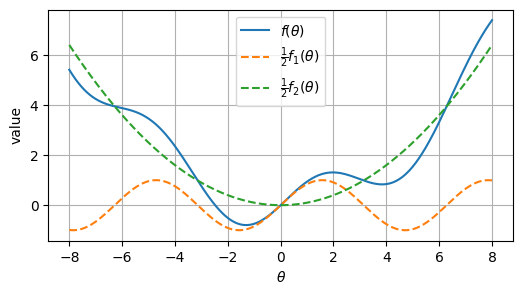
c = 0.1

def f1(theta):
    return 2 * np.sin(theta)

def f2(theta):
    return 2 * c * theta ** 2

def objective(theta):
    return 0.5 * (f1(theta) + f2(theta))

def grad_f1(theta):
    return 2 * np.cos(theta)

def grad_f2(theta):
    return 4 * c * theta

def grad_full(theta):
    return 0.5 * (grad_f1(theta) + grad_f2(theta))

def sample_gradient(theta, rng, batch_size=1):
    labels = rng.integers(0, 2, size=batch_size)
    gradients = np.where(labels == 0, grad_f1(theta), grad_f2(theta))
    return gradients.mean(), labels

theta_grid = np.linspace(-8, 8, 800)
plt.plot(theta_grid, objective(theta_grid), label=r'$f(\theta)$')
plt.plot(theta_grid, 0.5 * f1(theta_grid), '--', label=r'$\frac{1}{2} f_1(\theta)$')
plt.plot(theta_grid, 0.5 * f2(theta_grid), '--', label=r'$\frac{1}{2} f_2(\theta)$')
plt.xlabel(r'$\theta$')
plt.ylabel('value')
plt.legend()
plt.show()
2. 检查无偏性
下面固定一个 ,重复抽样很多次。样本平均值应接近完整梯度。
theta_demo = 2.0
rng = np.random.default_rng(SEED)
samples = np.array([sample_gradient(theta_demo, rng)[0] for _ in range(20_000)])

print('完整梯度:', round(float(grad_full(theta_demo)), 4))
print('随机梯度样本均值:', round(float(samples.mean()), 4))
print('随机梯度样本标准差:', round(float(samples.std()), 4))
完整梯度: -0.0161
随机梯度样本均值: -0.0187
随机梯度样本标准差: 0.8161
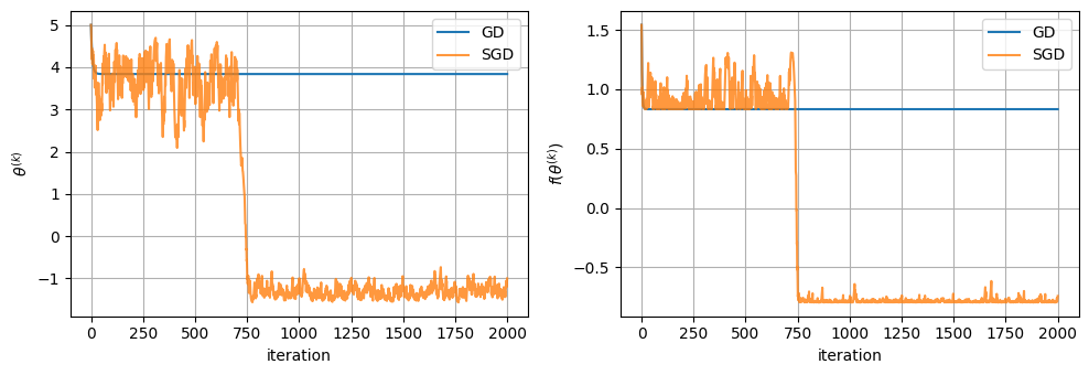
3. 比较 GD 与 SGD 的轨迹
完整梯度下降每步使用 。SGD 每步只随机选择一个分量梯度。下面的随机种子会展示一种典型现象:SGD 轨迹更抖,并且在这个例子中有机会离开右侧局部区域。这个现象有助于建立直觉,但不是一般收敛定理的保证。
def run_full_gradient(theta0, steps, lr):
    path = [theta0]
    theta = theta0
    for _ in range(steps):
        theta = theta - lr * grad_full(theta)
        path.append(theta)
    return np.array(path)


def run_stochastic_gradient(theta0, steps, lr, batch_size=1, seed=SEED):
    rng = np.random.default_rng(seed)
    path = [theta0]
    chosen_labels = []
    theta = theta0
    for _ in range(steps):
        gradient, labels = sample_gradient(theta, rng, batch_size=batch_size)
        theta = theta - lr * gradient
        path.append(theta)
        chosen_labels.extend(labels.tolist())
    return np.array(path), np.array(chosen_labels)

steps = 2_000
learning_rate = 0.15
theta0 = 5.0

gd_path = run_full_gradient(theta0, steps, learning_rate)
sgd_path, sgd_labels = run_stochastic_gradient(theta0, steps, learning_rate, seed=SEED)

gd_loss = objective(gd_path)
sgd_loss = objective(sgd_path)

print(f'GD final theta={gd_path[-1]:.3f}, loss={gd_loss[-1]:.3f}')
print(f'SGD final theta={sgd_path[-1]:.3f}, loss={sgd_loss[-1]:.3f}')
print(f'SGD chose component 2 about {sgd_labels.mean():.3f} of the time')
GD final theta=3.837, loss=0.832
SGD final theta=-0.999, loss=-0.741
SGD chose component 2 about 0.504 of the time
fig, axes = plt.subplots(1, 2, figsize=(10, 3.5))

axes[0].plot(gd_path, label='GD')
axes[0].plot(sgd_path, label='SGD', alpha=0.8)
axes[0].set_xlabel('iteration')
axes[0].set_ylabel(r'$\theta^{(k)}$')
axes[0].legend()

axes[1].plot(gd_loss, label='GD')
axes[1].plot(sgd_loss, label='SGD', alpha=0.8)
axes[1].set_xlabel('iteration')
axes[1].set_ylabel(r'$f(\theta^{(k)})$')
axes[1].legend()

plt.tight_layout()
plt.show()
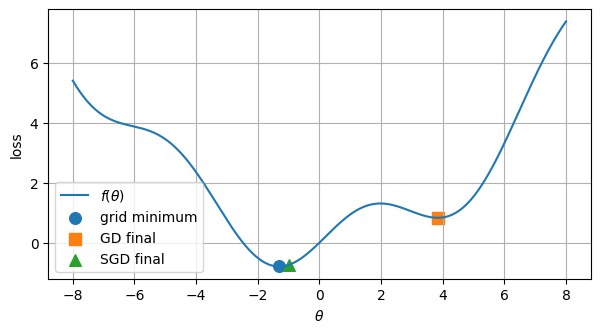
best_index = np.argmin(objective(theta_grid))
best_theta = theta_grid[best_index]
best_loss = objective(best_theta)

plt.figure(figsize=(7, 3.5))
plt.plot(theta_grid, objective(theta_grid), label=r'$f(\theta)$')
plt.scatter(best_theta, best_loss, label='grid minimum', s=70)
plt.scatter(gd_path[-1], gd_loss[-1], label='GD final', marker='s', s=70)
plt.scatter(sgd_path[-1], sgd_loss[-1], label='SGD final', marker='^', s=70)
plt.xlabel(r'$\theta$')
plt.ylabel('loss')
plt.legend()
plt.show()
4. Mini-batch SGD:batch size 与噪声
现在正式引入 mini-batch SGD。这里的目标只有两个分量,所以 batch size 大于 1 时可以理解为“有放回地多抽几次再平均”。batch size 越大,单次随机梯度的方差越小,方向通常越接近完整梯度;但每次更新也更贵,而且在非凸问题中不保证最终函数值一定更低。
part4_iterations = 7_000
learning_rate = 0.15
seed = 42

batch_runs = {
    'batch=1': \
        run_stochastic_gradient(theta0, part4_iterations, learning_rate, batch_size=1, seed=seed)[0],
    'batch=2': \
        run_stochastic_gradient(theta0, part4_iterations, learning_rate, batch_size=2, seed=seed)[0],
    'batch=4': \
        run_stochastic_gradient(theta0, part4_iterations, learning_rate, batch_size=4, seed=seed)[0],
    'full GD': \
        run_full_gradient(theta0, part4_iterations, learning_rate),
}

plt.figure(figsize=(7, 3.5))
for name, path in batch_runs.items():
    plt.plot(objective(path), label=name)
plt.xlabel('iteration')
plt.ylabel('loss')
plt.legend()
plt.show()

for name, path in batch_runs.items():
    print(f'{name:8s}: final theta={path[-1]: .3f}, final loss={objective(path[-1]): .3f}')
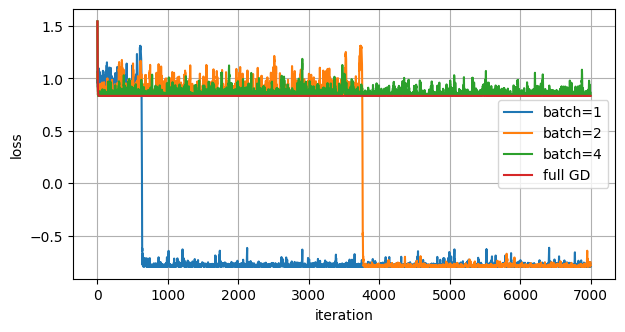
batch=1 : final theta=-1.305, final loss=-0.795
batch=2 : final theta=-1.046, final loss=-0.756
batch=4 : final theta= 4.095, final loss= 0.862
full GD : final theta= 3.837, final loss= 0.832
5. Logistic 回归:mini-batch 训练
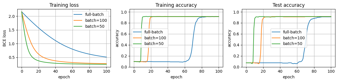
第8.1节中我们用 full-batch 训练 Logistic 回归。现在只改变 DataLoader 的 batch_size:full-batch 每个 epoch 更新一次,mini-batch 每个 epoch 会更新多次。因此按 epoch 画图时,mini-batch 曲线同时反映了“更多更新次数”和“随机梯度噪声”两个因素。训练集和测试集分开评估,测试准确率只在未参与训练的测试集上计算。
def make_binary_data(n_per_class, noise_count=0, seed=42, class_std=0.9):
    generator = torch.Generator().manual_seed(seed)
    class_0 = torch.randn(n_per_class, 2, generator=generator) * class_std + torch.tensor([-1.0, -1.0])
    class_1 = torch.randn(n_per_class, 2, generator=generator) * class_std + torch.tensor([1.0, 1.0])

    X = torch.cat([class_0, class_1])
    y = torch.cat([torch.zeros(n_per_class), torch.ones(n_per_class)])

    if noise_count > 0:
        noisy_index = torch.randperm(len(y), generator=generator)[:noise_count]
        y[noisy_index] = 1 - y[noisy_index]

    shuffle_index = torch.randperm(len(y), generator=generator)
    return X[shuffle_index], y[shuffle_index]


X_train, y_train = make_binary_data(200, noise_count=10, seed=42)
X_test, y_test = make_binary_data(100, noise_count=5, seed=43)
train_data = TensorDataset(X_train, y_train)
test_data = TensorDataset(X_test, y_test)
train_eval_loader = DataLoader(train_data, batch_size=len(train_data), shuffle=False)
test_loader = DataLoader(test_data, batch_size=len(test_data), shuffle=False)

criterion = nn.BCEWithLogitsLoss()

def predict_logits(X, a, b):
    return X @ a + b

def evaluate_logistic(data_loader, a, b):
    total_loss = 0.0
    total_correct = 0
    total_count = 0

    with torch.no_grad():
        for X_batch, y_batch in data_loader:
            logits = predict_logits(X_batch, a, b)
            loss = criterion(logits, y_batch)
            predictions = (torch.sigmoid(logits) >= 0.5).float()

            total_loss += loss.item() * len(y_batch)
            total_correct += (predictions == y_batch).sum().item()
            total_count += len(y_batch)

    return total_loss / total_count, total_correct / total_count


def train_logistic(batch_size, epochs=100, learning_rate=0.02, seed=SEED):
    generator = torch.Generator().manual_seed(seed)
    train_loader = DataLoader(train_data, batch_size=batch_size, shuffle=True, generator=generator)

    a = nn.Parameter(torch.tensor([-1.0, -1.0]))
    b = nn.Parameter(torch.zeros(()))
    optimizer = torch.optim.SGD([a, b], lr=learning_rate)

    train_losses = []
    train_accuracies = []
    test_accuracies = []

    train_loss, train_accuracy = evaluate_logistic(train_eval_loader, a, b)
    _, test_accuracy = evaluate_logistic(test_loader, a, b)
    train_losses.append(train_loss)
    train_accuracies.append(train_accuracy)
    test_accuracies.append(test_accuracy)

    for _ in range(epochs):
        for X_batch, y_batch in train_loader:
            optimizer.zero_grad()
            loss = criterion(predict_logits(X_batch, a, b), y_batch)
            loss.backward()
            optimizer.step()

        train_loss, train_accuracy = evaluate_logistic(train_eval_loader, a, b)
        _, test_accuracy = evaluate_logistic(test_loader, a, b)
        train_losses.append(train_loss)
        train_accuracies.append(train_accuracy)
        test_accuracies.append(test_accuracy)

    return train_losses, train_accuracies, test_accuracies


batch_sizes = {
    "full-batch": len(train_data),
    "batch=100": 100,
    "batch=50": 50,
}

logistic_runs = {}
for name, batch_size in batch_sizes.items():
    train_losses, train_accuracies, test_accuracies = train_logistic(batch_size=batch_size)
    logistic_runs[name] = {
        "train_loss": train_losses,
        "train_accuracy": train_accuracies,
        "test_accuracy": test_accuracies,
    }
    print(
        f"{name:10s}: initial test accuracy={test_accuracies[0]:.1%}, "
        f"final train accuracy={train_accuracies[-1]:.1%}, "
        f"final test accuracy={test_accuracies[-1]:.1%}"
    )

fig, axes = plt.subplots(1, 3, figsize=(12, 3))

for name, result in logistic_runs.items():
    axes[0].plot(result["train_loss"], label=name)
    axes[1].plot(result["train_accuracy"], label=name)
    axes[2].plot(result["test_accuracy"], label=name)

axes[0].set_title("Training loss")
axes[0].set_xlabel("epoch")
axes[0].set_ylabel("BCE loss")

axes[1].set_title("Training accuracy")
axes[1].set_xlabel("epoch")
axes[1].set_ylabel("accuracy")
axes[1].set_ylim(0, 1.05)

axes[2].set_title("Test accuracy")
axes[2].set_xlabel("epoch")
axes[2].set_ylabel("accuracy")
axes[2].set_ylim(0, 1.05)

for ax in axes:
    ax.legend()

plt.tight_layout()
plt.show()
full-batch: initial test accuracy=7.5%, final train accuracy=91.5%, final test accuracy=91.0%
batch=100 : initial test accuracy=7.5%, final train accuracy=91.5%, final test accuracy=91.5%
batch=50 : initial test accuracy=7.5%, final train accuracy=91.5%, final test accuracy=91.5%
6. 小结
随机梯度不是随便乱走,而是在无偏性假设下近似完整梯度;
SGD 的轨迹通常更抖,这正是随机梯度噪声的表现;
mini-batch SGD 通过平均多个样本梯度降低噪声;
增大 batch size 会降低噪声,但也会提高单次更新成本;
Logistic 回归中,减小 batch size 会让每个 epoch 内有更多次参数更新;
非凸问题中,噪声有时帮助探索,但不保证一定找到全局最优解。