3.1 梯度下降
目标:
知道梯度法的收敛速度在图像中的表现形式,即关于迭代次数呈现线性负相关,其中是第次迭代时候的误差
了解和对比精确直线搜索和回溯直线搜索的效果(从性能和所需要的时间角度出发)
回溯直线搜索中参数的影响
了解问题中不同方向的拉伸程度(即条件数)对于收敛速度的影响
不同坐标系变换下的最速下降法的对比
import numpy as np
import matplotlib.pyplot as plt
from scipy.optimize import minimize_scalar
import time

# 设置 matplotlib 正常显示中文和负号
plt.rcParams['font.sans-serif'] = ['Arial Unicode MS', 'PingFang SC',\
     'Heiti TC', 'SimHei']
plt.rcParams['axes.unicode_minus'] = False
import os
os.makedirs('assets', exist_ok=True)def exact_line_search(prob, x, d):
"""
Exact line search along the direction d
"""
phi = lambda t: prob.f(x + t * d)
result = minimize_scalar(phi, method='Golden')
return result.x
def backtracking_line_search(prob, x, d, alpha=0.1, beta=0.8):
"""
Backtracking line search (Armijo condition)
"""
k = 0
t = 1.0
fx = prob.f(x)
rate = np.dot(prob.df(x), d)
while prob.f(x + t * d) > fx + t * alpha * rate:
t *= beta
k += 1
return t, kclass ProblemEg1:
def __init__(self, γ=2.0, linesearch="exact", alpha=0.1, beta=0.8):
self.γ = γ
self.linesearch = linesearch
self.alpha = alpha
self.beta = beta
self.tol = 1.0e-6
self.ref_state = np.zeros(2) # 对该问题,我们有真解
self.condition = "grad" # 停止条件
self.P = np.eye(2) # 默认无坐标变换
def f(self, x):
"""
objective function f.
"""
return (x[0]**2 + self.γ * x[1]**2) / 2
def df(self, x):
"""
gradient of f
"""
return np.array([x[0], self.γ * x[1]])
def gradient_propose(self, x):
# 如果P是单位阵,这就是负梯度方向
return - np.linalg.solve(self.P, self.df(x))
def update(self, x):
# 迭代更新一步
d = self.gradient_propose(x)
if self.linesearch == "exact":
t = exact_line_search(self, x, d)
elif self.linesearch == "backtracking":
t, _ = backtracking_line_search(
self, x, d,
alpha=self.alpha,
beta=self.beta
)
else:
raise ValueError("Unknown linesearch method")
return x + t * d
def stop_condition(self, x):
# 停止条件的判断
if self.condition == "ref_state":
return np.linalg.norm(x - self.ref_state) < self.tol
elif self.condition == "grad":
return np.linalg.norm(self.df(x)) < self.tol
else:
raise ValueError("Unknown stopping condition")
def solve(self, x0, max_iter=100, num_repeat=1):
t_begin = time.time()
for _ in range(num_repeat): # 需要num_repeat仅为了稳定估计运行时间
x = x0.copy()
trajectory = [x.copy()]
for _ in range(max_iter):
x = self.update(x)
trajectory.append(x.copy())
# 终止条件
if self.stop_condition(x):
break
runtime = (time.time() - t_begin) / num_repeat
return np.array(trajectory), runtime
def plot_contour(self, xmin, xmax, ymin, ymax):
grid_x = np.linspace(xmin, xmax, 400)
grid_y = np.linspace(ymin, ymax, 300)
grid_X, grid_Y = np.meshgrid(grid_x, grid_y)
# 利用numpy的广播机制向量化计算Z
Z = (grid_X**2 + self.γ * grid_Y**2) / 2
contour = plt.contourf(
grid_X, grid_Y, Z,
levels=20, cmap='Blues'
)
plt.colorbar(contour)
plt.xlabel(r'$x_1$', fontsize=12)
plt.ylabel(r'$x_2$', fontsize=12)探究迭代法收敛的表现形式
γ = 10.0
x0 = np.array([9.0, 2.0])

# γ = 20.0
# x0 = np.array([7.0, 3.0])

xmin = -5; xmax = 10; ymin = -5; ymax = 5
ls = "exact"
alpha = 0.1
beta = 0.8
prob = ProblemEg1(
    γ=γ, linesearch=ls,
    alpha=alpha, beta=beta
)
num_repeat = 20 # 重复实验的次数,为了估计运行时间的结果的稳定

# 精确直线搜索
prob.linesearch = "exact"
trajectory_exact, runtime = prob.solve(x0, num_repeat=num_repeat)
print("ELS uses {:.2E} seconds".format(runtime))

# 回溯直线搜索
prob.linesearch = "backtracking"
trajectory_backtracking, runtime = prob.solve(x0, num_repeat=num_repeat)
print("BLS uses {:.2E} seconds".format(runtime))

# Plot the results
plt.figure(figsize=(10, 4.5))

# 子图 1:迭代轨迹
plt.subplot(1, 2, 1)
plt.plot(
    trajectory_exact[:, 0],
    trajectory_exact[:, 1],
    'ko-', label='精确搜索'
)
plt.plot(
    trajectory_backtracking[:, 0],
    trajectory_backtracking[:, 1],
    'rx-',
    label='回溯搜索'
)
prob.plot_contour(xmin, xmax, ymin, ymax)
plt.title("梯度下降法的迭代轨迹", fontsize=14)
plt.legend(fontsize=12)

# 子图 2:误差下降曲线
plt.subplot(1, 2, 2)
plt.plot(
    np.linalg.norm(trajectory_exact, ord=2, axis=1),
    'ko-', label='精确搜索'
)
plt.plot(
    np.linalg.norm(trajectory_backtracking, ord=2, axis=1),
    'rx-',
    label='回溯搜索'
)
plt.yscale('log')
plt.title("梯度下降法的误差收敛", fontsize=14)
plt.xlabel("迭代步数", fontsize=12)
plt.ylabel("误差 (到原点距离)", fontsize=12)
plt.legend(fontsize=12)
plt.grid()
plt.tight_layout()

plt.savefig('assets/trajectory_comparison.pdf', bbox_inches='tight')

plt.show()
ELS uses 5.14E-03 seconds
BLS uses 1.91E-03 seconds
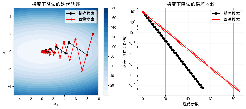
对于该问题,观察到的情况:
对于相同的迭代步数,精确线性搜索大概率可以提高精度。
但是从实际效果来看,达到同样的精度,精确线性搜索可能需要更多的计算时间。
这些结论只是经验结论。
探究回溯直线搜索中参数的影响
关于 和 参数的实验说明
回溯直线搜索(Armijo条件控制)中包含两个核心参数:
:接受步长的阈值因子。 越大,表示对函数值下降程度的要求越苛刻(迫使在这一步下降更多)。通常 取值较小,如
0.01到0.3。:步长回溯的缩放因子。当步长不满足Armijo条件时,下一步测试的步长缩减为 。 值较大(如
0.8、0.9)意味着回溯更加精细,但可能需要更多次的函数求值试探; 较小(如0.5)会导致很快缩小步长,从而可以更快找到一个满足条件的较小步长,但可能导致整体迭代次数增加。
在接下来的代码中,我们会可视化展示在这两个参数的不同取值组合下,误差 (Error)、迭代步数 (Iteration Steps),以及 总运行时间 (Runtime) 随参数的变化趋势。
def effect_of_alpha_and_beta(alpha, beta, x0, max_iter, gamma=10.0):

    ls = "backtracking"
    prob = ProblemEg1(
        γ=gamma, linesearch=ls,
        alpha=alpha, beta=beta
    )

    prob.condition = "ref_state"
    prob.tol = 1.0e-5
    traj, runtime = prob.solve(x0, max_iter=max_iter)

    iter_step = traj.shape[0] - 1
    final_state = traj[-1, :]
    err = np.linalg.norm(final_state)  # 如此计算是因为此处的真解是[0,0]

    return err, iter_step, runtime
def visualize_effect_alpha_beta(beta_list, max_iter=200):
"""
可视化探索回溯直线搜索在不同的 alpha 和 beta 组合下,
最终误差、迭代步数,以及运行时间的关系。
"""
x0 = np.array([5.0, 6.0]) # 本次实验固定的初始值
# 在 [0.01, 0.96] 区间里取 20 个不同的 alpha 进行测试
alpha_list = np.linspace(0.01, 0.96, 20)
gamma = 10.0 # 固定系数 gamma 用来探究参数影响
# 针对每一个给定的回溯衰减参数 beta 循环作图
for i, beta in enumerate(beta_list):
err_list = np.zeros(len(alpha_list))
iter_list = np.zeros(len(alpha_list))
runtime_list = np.zeros(len(alpha_list))
# 对于当前 beta,循环遍历所有的 alpha 以记录性能指标
for j, alpha in enumerate(alpha_list):
err_list[j], iter_list[j], runtime_list[j] = \
effect_of_alpha_and_beta(alpha, beta, x0, max_iter, gamma)
# ====== 绘图:最终结果误差 ======
plt.subplot(1, 3, 1)
plt.plot(alpha_list, err_list, 'o-.', label=rf"$\beta={beta:.2f}$")
plt.ylim([10**-6, 10**-3])
plt.yscale("log") # 对数图更能反映误差的量级
if i == len(beta_list) - 1:
plt.xlabel(r"$\alpha$", fontsize=14)
plt.title('误差\n(最终误差越小越好)', fontsize=16)
# ====== 绘图:迭代步数 ======
plt.subplot(1, 3, 2)
plt.plot(alpha_list, iter_list, 'o-.', label=rf"$\beta={beta:.2f}$")
plt.ylim([0, max_iter])
if i == len(beta_list) - 1:
plt.xlabel(r"$\alpha$", fontsize=14)
plt.title('迭代步数\n(所需步数越少越好)', fontsize=16)
# ====== 绘图:程序运行时间 ======
plt.subplot(1, 3, 3)
plt.plot(
alpha_list,
runtime_list * 1000,
'o-.',
label=rf"$\beta={beta:.2f}$"
)
plt.ylim([0, 10])
if i == len(beta_list) - 1:
plt.xlabel(r"$\alpha$", fontsize=14)
plt.title('运行时间 (ms)\n(越快越好)', fontsize=16)
plt.legend(fontsize=12)
plt.tight_layout()beta_list = [0.05]
plt.figure(figsize=(12, 4))
visualize_effect_alpha_beta(beta_list)
plt.savefig('assets/alpha_beta_effect_1.pdf', bbox_inches='tight')
plt.show()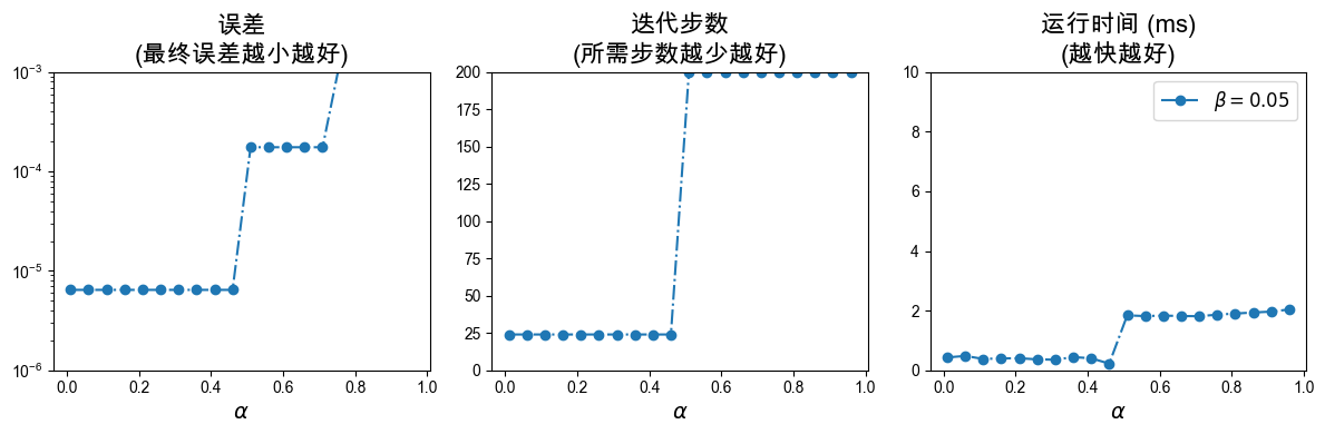
beta_list = [0.2, 0.6, 0.9]
plt.figure(figsize=(12, 4))
visualize_effect_alpha_beta(beta_list)
plt.savefig('assets/alpha_beta_effect_2.pdf', format='pdf', bbox_inches='tight')
plt.show()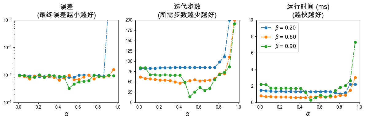
beta_list = [0.95]
plt.figure(figsize=(12, 4))
visualize_effect_alpha_beta(beta_list)
plt.savefig('assets/alpha_beta_effect_3.pdf', bbox_inches='tight')
plt.show()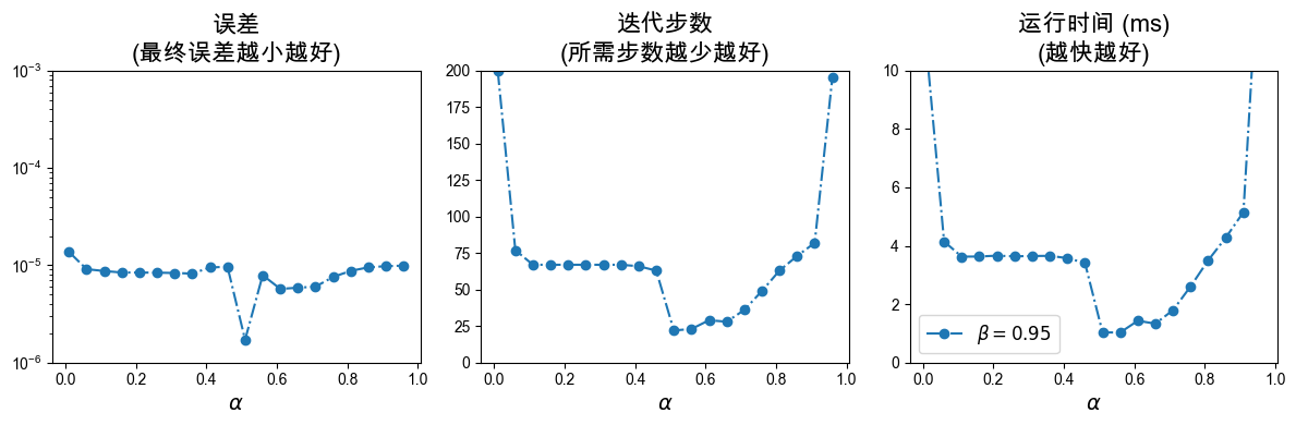
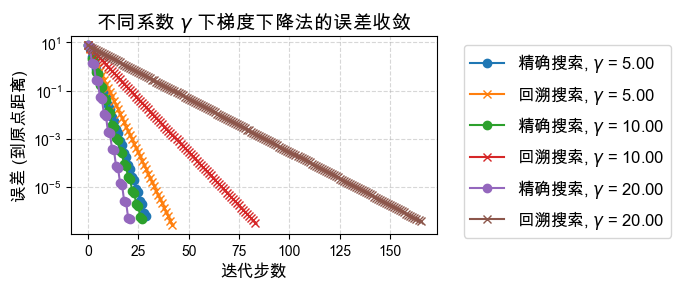
探究问题本身对于迭代次数的影响,即系数 
对于目标函数 ,参数 决定了等高线的形状(椭圆的扁平程度):
当 时,等高线为正圆,梯度总是直接指向极小值点,收敛应该非常快。
当 偏离 1 越大(无论很大还是趋于 0),等高线越呈极其扁平的椭圆,目标函数的Hessian矩阵的条件数越大,这就是所谓问题的“病态” (Ill-conditioned)。
优化这种病态问题时,典型的梯度下降法会在“峡谷”的两壁之间来回震荡,导致收敛极为缓慢。
下面我们测试不同 取值对 精确直线搜索(ELS) 和 回溯直线搜索(BLS) 的影响。
def effect_of_gamma(γ, x0):
"""
可视化测试在给定的目标函数系数 gamma 条件下,
精确直线搜索 (ELS) 与 回溯直线搜索 (BLS) 的收敛速度对比。
"""
max_iter = 200
alpha = 0.1
beta = 0.8
num_repeat = 10 # 重复实验的次数,为了使得最后估计的运行时间结果更稳定
# ------ 测试 1:精确直线搜索 (ELS) ------
ls_exact = "exact"
prob_exact = ProblemEg1(
γ=γ, linesearch=ls_exact,
alpha=alpha, beta=beta
)
trajectory_exact, runtime_exact = prob_exact.solve(
x0, max_iter=max_iter, num_repeat=num_repeat
)
print("γ = " + f"{γ:5.2f}, ELS uses {runtime_exact:.2E} seconds")
# ------ 测试 2:回溯直线搜索 (BLS) ------
ls_backtracking = "backtracking"
prob_bls = ProblemEg1(
γ=γ, linesearch=ls_backtracking,
alpha=alpha, beta=beta
)
trajectory_backtracking, runtime_bls = prob_bls.solve(
x0, max_iter=max_iter, num_repeat=num_repeat
)
print("γ = " + f"{γ:5.2f}, BLS uses {runtime_bls:.2E} seconds")
# ====== 绘制这两种方法在当前 gamma 下的误差下降曲线 ======
plt.plot(
np.linalg.norm(trajectory_exact, ord=2, axis=1),
'o-',
label=r'精确搜索, $\gamma$' + f' = {γ:.2f}'
)
plt.plot(
np.linalg.norm(trajectory_backtracking, ord=2, axis=1),
'x-',
label=r'回溯搜索, $\gamma$' + f' = {γ:.2f}'
)
plt.yscale('log')
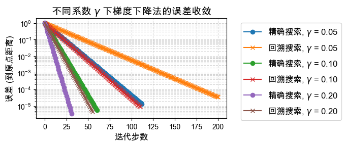
plt.title(r'不同系数 $\gamma$ 下梯度下降法的误差收敛', fontsize=14)
plt.xlabel('迭代步数', fontsize=12)
plt.ylabel('误差 (到原点距离)', fontsize=12)
# 将图例放在图的外部,避免遮挡曲线
plt.legend(bbox_to_anchor=(1.05, 1.0), fontsize=12)
plt.grid(True, which="both", ls="--", alpha=0.5)plt.figure(figsize=(7, 3))
effect_of_gamma(0.05, np.array([0.05, 1])); print()
effect_of_gamma(0.10, np.array([0.10, 1])); print()
effect_of_gamma(0.20, np.array([0.20, 1])); print()
plt.tight_layout()
plt.savefig('assets/effect_of_gamma_small.pdf', bbox_inches='tight')
plt.show()γ = 0.05, ELS uses 1.01E-02 seconds
γ = 0.05, BLS uses 2.38E-03 seconds
γ = 0.10, ELS uses 5.43E-03 seconds
γ = 0.10, BLS uses 1.29E-03 seconds
γ = 0.20, ELS uses 2.77E-03 seconds
γ = 0.20, BLS uses 6.57E-04 seconds
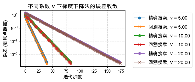
plt.figure(figsize=(7, 3))
effect_of_gamma(5.00, np.array([5.00, 1])); print()
effect_of_gamma(10.00, np.array([10.00, 1])); print()
effect_of_gamma(20.00, np.array([20.00, 1])); print()
plt.tight_layout()
plt.savefig('assets/effect_of_gamma_large.pdf', bbox_inches='tight')
plt.show()
γ = 5.00, ELS uses 3.79E-03 seconds
γ = 5.00, BLS uses 7.75E-04 seconds
γ = 10.00, ELS uses 8.09E-03 seconds
γ = 10.00, BLS uses 1.94E-03 seconds
γ = 20.00, ELS uses 1.71E-02 seconds
γ = 20.00, BLS uses 4.54E-03 seconds
探究初值对迭代效果的影响
梯度下降的收敛速度同样强烈依赖于初始猜测点 :
初值的方向:如果初始点恰好位于是长轴或短轴(对于二次型而言),梯度方向可能会直接指向或高度吻合指向最低点,那么一步或几步就能收敛。
震荡的影响:如果初值点落在导致锯齿状震荡的“峡谷”山腰线上,迭代步数会急剧增加。
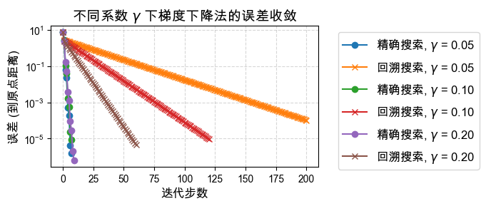
下面我们给出一个新的初值 ,来观察收敛曲线是否和上方有所区别。
x0 = np.array([7.0, 3.0]) # 新的初始猜测点 Initial guess

plt.figure(figsize=(7,3))
effect_of_gamma(0.05, x0.copy()); print()
effect_of_gamma(0.10, x0.copy()); print()
effect_of_gamma(0.20, x0.copy()); print()
plt.tight_layout()
plt.savefig('assets/effect_of_gamma_small_x0.pdf', bbox_inches='tight')
plt.show()
γ = 0.05, ELS uses 6.71E-04 seconds
γ = 0.05, BLS uses 2.40E-03 seconds
γ = 0.10, ELS uses 6.62E-04 seconds
γ = 0.10, BLS uses 1.42E-03 seconds
γ = 0.20, ELS uses 8.36E-04 seconds
γ = 0.20, BLS uses 7.17E-04 seconds
# 对比大于 1 的 gamma (问题会在 y 方向拉伸)
plt.figure(figsize=(7, 3))
effect_of_gamma(5.0, x0.copy()); print()
effect_of_gamma(10.0, x0.copy()); print()
effect_of_gamma(20.0, x0.copy()); print()
plt.tight_layout()
plt.savefig('assets/effect_of_gamma_large_x0.pdf', bbox_inches='tight')
plt.show()
γ = 5.00, ELS uses 2.79E-03 seconds
γ = 5.00, BLS uses 8.17E-04 seconds
γ = 10.00, ELS uses 2.62E-03 seconds
γ = 10.00, BLS uses 1.87E-03 seconds
γ = 20.00, ELS uses 2.06E-03 seconds
γ = 20.00, BLS uses 4.34E-03 seconds
最速下降法与不同坐标系(度量)的影响
普通的梯度下降法 实质上是在标准欧几里得范数意义下的最速下降。 当问题的条件数很大时(例如上面出现的震荡情况),欧氏空间中的梯度并不指向真正的极小值。
为了克服这一问题,我们可以改变“坐标系”(或者是范数矩阵),使用 -范数定义下的最速下降方向:
这里矩阵 扮演着尺度拉伸的角色:
当 (单位矩阵)时,退化为普通的梯度下降。
如果我们能聪明地选择 (例如取目标函数的 Hessian 矩阵,这就会演变成牛顿法;见后面第三节), 将使得转换后的坐标系中等高线变圆,消除原本空间里的病态问题,从而实现只需要极少步便可极快收敛。
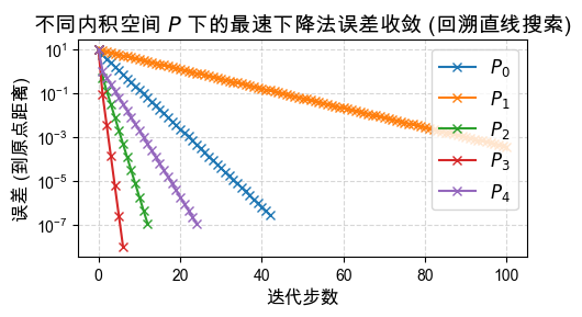
以下展示在这 5 种不同的尺度矩阵 缩放下:
问题的收敛行为。你能发现哪个 的表现最好,为什么吗?
# 固定 γ 为一个病态情形的值,比如 5.0
γ = 5.0
x0 = np.array([9.0, 2.0])

# 设计各种不同的坐标系度量矩阵 P
Plist = [
    np.eye(2),                       # P_0: 退化为标准梯度下降
    np.array([[1, 0], [0, 1/4]]),    # P_1: 错误方向的缩放
    np.array([[1, 0], [0, 4]]),      # P_2: 正确但还不够的缩放
    np.array([[1, 0], [0, 4.8]]),    # P_3: 非常接近最优缩放
    np.array([[1, 0], [0, 10]])      # P_4: 缩放过度
]

plt.figure(figsize=(5, 3))

# 遍历每一个给定的 P 矩阵
for P_idx, P in enumerate(Plist):
    ls = "exact" # 统一使用精确直线搜索
    prob = ProblemEg1(
        γ=γ, linesearch=ls,
        alpha=0.1, beta=0.8
    )
    prob.P = P # 覆盖默认的 P = I,替换为新的尺度矩阵
    trajectory_exact, _ = prob.solve(x0)

    # 绘制当前尺度矩阵下的误差下降曲线
    plt.plot(
        np.linalg.norm(trajectory_exact, ord=2, axis=1),
        'o-',
        label=rf'$P_{P_idx}$'
    )

plt.yscale('log')
plt.title(
    r"不同内积空间 $P$ 下的最速下降法误差收敛 (精确直线搜索)",
    fontsize=14
)
plt.xlabel("迭代步数", fontsize=12)
plt.ylabel('误差 (到原点距离)', fontsize=12)
plt.legend(fontsize=12)

plt.grid(True, which="both", ls="--", alpha=0.5) # 增加横纵辅助线
plt.tight_layout()

plt.savefig('assets/steepest_descent_exact.pdf', bbox_inches='tight')

plt.show()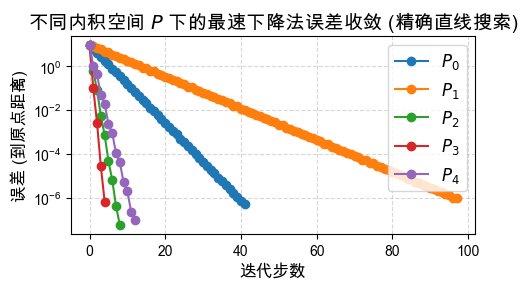
plt.figure(figsize=(5, 3))

# 遍历每一个给定的 P 矩阵
for P_idx, P in enumerate(Plist):
    ls = "backtracking" # 统一使用回溯直线搜索
    prob = ProblemEg1(
        γ=γ, linesearch=ls,
        alpha=0.1, beta=0.8
    )
    prob.P = P # 替换尺度矩阵
    trajectory_backtracking, _ = prob.solve(x0)

    # 绘制当前尺度矩阵下的误差下降曲线
    plt.plot(
        np.linalg.norm(trajectory_backtracking, ord=2, axis=1),
        'x-',
        label=rf'$P_{P_idx}$'
    )

plt.yscale('log')
plt.title(
    r"不同内积空间 $P$ 下的最速下降法误差收敛 (回溯直线搜索)",
    fontsize=14
)
plt.xlabel("迭代步数", fontsize=12)
plt.ylabel('误差 (到原点距离)', fontsize=12)
plt.legend(fontsize=12, loc='upper right')

plt.grid(True, which="both", ls="--", alpha=0.5) # 增加横纵辅助线
plt.tight_layout()

plt.savefig('assets/steepest_descent_backtracking.pdf', bbox_inches='tight')

plt.show()