6.1 等式约束的牛顿法

import numpy as np
import cvxpy as cp
import matplotlib.pyplot as plt

class EqualityConstrainedProblem:
    # 将目标函数、导数、Hessian 和等式约束 Ax=b 封装在同一个类中。
    def __init__(self, f, df, hess, A, b, is_in_domain=None):
        # is_in_domain 用来检查目标函数定义域；本例中要求所有坐标都为正。
        self.f = f
        self.df = df
        self.hess = hess
        self.A = np.asarray(A, dtype=float)
        self.b = np.asarray(b, dtype=float)
        self.p, self.n = self.A.shape
        self.is_in_domain = is_in_domain or (lambda x: True)

        # 约束数量必须和 b 的长度一致。
        if self.b.shape != (self.p,):
            raise ValueError("b must have shape (p,).")

    def newton_step(self, x, nu=None):
        # 求解课件中的 KKT 线性方程组，得到 Newton 方向。
        # 可行初始点方法只需要 dx；不可行初始点方法还需要 dnu。
        if not self.is_in_domain(x):
            raise ValueError("Newton step is only defined inside the domain of f.")

        n = self.n
        p = self.p
        # KKT 矩阵为 [[H, A^T], [A, 0]]，其中 H 是 Hessian。
        kkt_matrix = np.zeros((n + p, n + p))
        kkt_matrix[:n, :n] = self.hess(x)
        kkt_matrix[:n, n:] = self.A.T
        kkt_matrix[n:, :n] = self.A

        # 右端向量对应 [-grad f(x), b - A x]。
        rhs = np.zeros(n + p)
        rhs[:n] = -self.df(x)
        rhs[n:] = self.b - self.A @ x

        solution = np.linalg.solve(kkt_matrix, rhs)
        dx = solution[:n]
        omega = solution[n:]

        if nu is not None:
            # 不可行初始点方法中，KKT 解给出 omega = nu + dnu。
            return dx, omega - nu
        return dx

    def primal_residual(self, x):
        # 衡量当前点违反等式约束 Ax=b 的程度。
        return np.linalg.norm(self.A @ x - self.b)

    def backtracking_line_search(self, x, dx, alpha, beta, max_line_search=100):
        # Armijo 回溯线搜索：既要求函数下降，也要求试探点仍在定义域内。
        fx = self.f(x)
        directional_derivative = np.dot(self.df(x), dx)
        t = 1.0

        for k in range(max_line_search + 1):
            xt = x + t * dx
            if self.is_in_domain(xt):
                # 先检查定义域，再计算 f(xt)，避免 log 遇到非正数。
                sufficient_decrease = self.f(xt) <= fx + alpha * t * directional_derivative
                if sufficient_decrease:
                    return t, k
            t *= beta

        raise RuntimeError("Line search failed to find a domain-feasible step.")

    def newton_with_linear_constraint(self, x, alpha, beta, epsilon, maxiter=100):
        # 可行初始点 Newton 法：要求初始点已经满足 Ax=b。
        x = np.asarray(x, dtype=float).copy()
        if self.primal_residual(x) > 1.0e-10:
            raise ValueError("Feasible-start Newton needs A @ x == b.")

        x_list = [x.copy()]
        for _ in range(maxiter):
            dx = self.newton_step(x)
            # Newton decrement 的平方：lambda(x)^2 = dx^T H dx。
            lambda_sq = np.dot(dx, self.hess(x) @ dx)
            if lambda_sq / 2 <= epsilon:
                break

            # 因为 A dx=0，任意步长都会保持 Ax=b；线搜索只负责下降和定义域。
            t, _ = self.backtracking_line_search(x, dx, alpha, beta)
            x = x + t * dx
            x_list.append(x.copy())
        return x, x_list

    def r(self, x, nu):
        # 原对偶残差 r(x, nu)，同时包含驻点误差和可行性误差。
        if not self.is_in_domain(x):
            return np.inf

        residual = (
            np.linalg.norm(self.df(x) + self.A.T @ nu) ** 2
            + self.primal_residual(x) ** 2
        )
        return np.sqrt(residual)

    def newton_with_infeasible_start(
        self, x, nu, alpha, beta, epsilon, eta=None, maxiter=100, max_line_search=100
    ):
        # 不可行初始点 Newton 法：x 不必满足 Ax=b，但必须在 f 的定义域内。
        # eta 是单独的可行性阈值；若不指定，则默认和 epsilon 相同。
        eta = epsilon if eta is None else eta
        x = np.asarray(x, dtype=float).copy()
        nu = np.asarray(nu, dtype=float).copy()
        x_list = [x.copy()]
        nu_list = [nu.copy()]

        for _ in range(maxiter):
            r0 = self.r(x, nu)
            # 同时检查 KKT 残差和等式约束残差，对应课件中的两个停止条件。
            if r0 <= epsilon and self.primal_residual(x) <= eta:
                break

            dx, dnu = self.newton_step(x, nu=nu)
            t = 1.0
            for _ in range(max_line_search + 1):
                xt = x + t * dx
                nut = nu + t * dnu
                if self.is_in_domain(xt):
                    # 这里用残差下降作为线搜索标准，而不是直接比较目标函数值。
                    residual_decrease = self.r(xt, nut) <= (1 - alpha * t) * r0
                    if residual_decrease:
                        break
                t *= beta
            else:
                raise RuntimeError(
                    "Line search failed to find a domain-feasible residual-decreasing step."
                )

            x = x + t * dx
            nu = nu + t * dnu
            x_list.append(x.copy())
            nu_list.append(nu.copy())

        return x, x_list, nu, nu_list

np.random.seed(1)

n = 500
p = 100
A = np.random.rand(p, n)
assert np.linalg.matrix_rank(A) == p, "Not full rank"
x0 = np.random.rand(n)
b = A @ x0

cp_x = cp.Variable(n)
constraints = [A @ cp_x == b]
obj = cp.Minimize(-cp.sum(cp.log(cp_x)))
cvx_prob = cp.Problem(obj, constraints)
cvx_prob.solve()
print("status:", cvx_prob.status)
print("optimal value = {:.4f}".format(cvx_prob.value))

alpha = 0.1
beta = 0.5
tol = 1.0e-7
eta = 1.0e-8

def is_positive(x):
    # log barrier 的定义域：每个坐标都必须大于 0。
    return np.all(x > 0)

def f(x):
    # 目标函数 f(x) = -sum log(x_i)，定义域外返回无穷大。
    if not is_positive(x):
        return np.inf
    return -np.sum(np.log(x))

def df(x):
    # 梯度：第 i 个分量为 -1 / x_i。
    return -1/x

def hess(x):
    # Hessian 是对角矩阵，第 i 个对角元为 1 / x_i^2。
    return np.diag(1/x**2)

problem = EqualityConstrainedProblem(f, df, hess, A, b, is_in_domain=is_positive)

final_x_ln, x_list_ln = problem.newton_with_linear_constraint(x0, alpha, beta, tol)

p_star_ln = f(final_x_ln)
print("Optimal value = {:.4f}".format(p_star_ln))
print("Iterations = {}".format(len(x_list_ln) - 1))
print("Final feasibility residual = {:.2e}".format(problem.primal_residual(final_x_ln)))

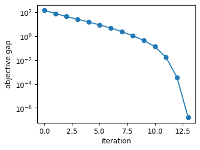
plt.figure(figsize=(4,3))
objective_gaps = [max(f(item) - p_star_ln, np.finfo(float).tiny) for item in x_list_ln[:-1]]
plt.semilogy(objective_gaps, 'o-')
plt.xlabel("iteration")
plt.ylabel("objective gap")

x0_infeasible = 0.5 * x0 + 0.1
nu0 = np.random.randn(p)

print("Initial feasibility residual = {:.2e}".format(problem.primal_residual(x0_infeasible)))
final_x_pd, x_list_pd, final_nu_pd, nu_list_pd = problem.newton_with_infeasible_start(
    x0_infeasible, nu0, alpha, beta, tol, eta=eta
)

p_star_pd = f(final_x_pd)
print("Optimal value = {:.4f}".format(p_star_pd))
print("Iterations = {}".format(len(x_list_pd) - 1))
print("Final KKT residual = {:.2e}".format(problem.r(final_x_pd, final_nu_pd)))
print("Final feasibility residual = {:.2e}".format(problem.primal_residual(final_x_pd)))

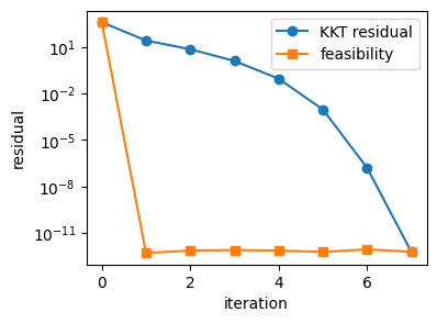
plt.figure(figsize=(4,3))
kkt_residuals = [problem.r(x, nu) for x, nu in zip(x_list_pd, nu_list_pd)]
feasibility_residuals = [problem.primal_residual(x) for x in x_list_pd]
plt.semilogy(kkt_residuals, 'o-', label="KKT residual")
plt.semilogy(feasibility_residuals, 's-', label="feasibility")
plt.xlabel("iteration")
plt.ylabel("residual")
plt.legend()

def relative_error(x, x_ref):
    return np.linalg.norm(x - x_ref) / np.linalg.norm(x_ref)

print("Compare cvxpy and newton (with linear constraints)")
print("Relative error of optimal x = {:.1E}".format(relative_error(final_x_ln, cp_x.value)))
print("Minimum coordinate of x = {:.2e}\n".format(np.min(final_x_ln)))

print("Compare cvxpy and newton (with infeasible start)")
print("Relative error of optimal x = {:.1E}".format(relative_error(final_x_pd, cp_x.value)))
print("Minimum coordinate of x = {:.2e}".format(np.min(final_x_pd)))