7.2 原对偶内点法 - MATH3806 Code

这个 notebook 与第7章第2部分“原对偶内点法”对应。为了让代码尽量直接，我们先看一个一维线性规划例子，再看一个 100 维线性规划例子，并直接实现原对偶牛顿方向。

本例重点观察：

原对偶残差 $r_{\mathrm{dual}}$ 和中心残差 $r_{\mathrm{cent}}$ ；
牛顿方向如何同时更新原变量 $x$ 和对偶乘子 $\lambda$ ；
线搜索如何保持严格可行性和 $\lambda>0$ ；
代理对偶间隙 $\hat\eta$ 如何趋近于 0；
高维 LP 例子中的迭代次数和运行时间。

import time

import numpy as np
import matplotlib.pyplot as plt

from IPython.display import HTML, display

plt.rcParams["font.sans-serif"] = [
    "Arial Unicode MS",
    "PingFang SC",
    "Heiti TC",
    "Microsoft YaHei",
    "SimHei",
]
plt.rcParams["axes.unicode_minus"] = False

print_large = lambda text: display(HTML(f'<font size="3">{text}</font>'))

一个简单例子¶

考虑一维问题

\begin{array}{ll} \text{minimize} & x \\ \text{subject to} & 1-x\le 0,\\ & x-2\le 0. \end{array}

(1)

也就是在区间 $1\le x\le 2$ 上最小化 $x$ 。原问题的最优解是

x^\star=1,\qquad p^\star=1.

(2)

两个不等式函数为

f_1(x)=1-x,\qquad f_2(x)=x-2.

(3)

算法从严格可行点 $1<x<2$ 和正乘子 $\lambda_1,\lambda_2>0$ 出发。

def f_constraints(x):
    return np.array([1.0 - x, x - 2.0])


def df_constraints(x):
    return np.array([-1.0, 1.0])


def objective(x):
    return x


x_star = 1.0
p_star = objective(x_star)
m = 2

print_large(f"原问题最优解 x* = {x_star:.1f}")
print_large(f"原问题最优值 p* = {p_star:.1f}")
print_large(f"点 x=1.5 的约束值 f(x) = {f_constraints(1.5)}")

原对偶残差¶

对给定的障碍参数 $t$ ，扰动 KKT 方程为

\begin{aligned} 1-\lambda_1+\lambda_2 &= 0,\\ -\lambda_i f_i(x) &= \frac{1}{t},\quad i=1,2. \end{aligned}

(4)

因此残差可以写成

r_{\mathrm{dual}} = 1-\lambda_1+\lambda_2,

(5)

r_{\mathrm{cent}} = -\operatorname{diag}(\lambda) f(x)-\frac{1}{t}\mathbf{1}.

(6)

本例没有等式约束，所以没有 $r_{\mathrm{pri}}$ 。

def residual(x, lam, t):
    r_dual = np.array([1.0 + df_constraints(x) @ lam])
    r_cent = -lam * f_constraints(x) - np.ones(m) / t
    return np.concatenate([r_dual, r_cent])


def surrogate_gap(x, lam):
    return -f_constraints(x) @ lam


def is_strictly_feasible(x, lam):
    return np.all(f_constraints(x) < 0) and np.all(lam > 0)

原对偶牛顿方向¶

对残差方程线性化，求解

J \begin{bmatrix} \Delta x\\ \Delta\lambda \end{bmatrix} =-r_t(x,\lambda).

(7)

因为本例的 $f_0,f_1,f_2$ 都是线性的，Lagrange 函数 Hessian 为 0，Newton 系统特别简单。

def primal_dual_direction(x, lam, t):
    f = f_constraints(x)
    df = df_constraints(x)
    r = residual(x, lam, t)

    jacobian = np.zeros((3, 3))
    jacobian[0, 1:] = df
    jacobian[1:, 0] = -lam * df
    jacobian[1:, 1:] = np.diag(-f)

    step = np.linalg.solve(jacobian, -r)
    dx = step[0]
    dlam = step[1:]
    return dx, dlam

运行原对偶内点法¶

每一步使用代理对偶间隙

\hat\eta=-f(x)^T\lambda

(8)

来选择

t=\frac{\mu m}{\hat\eta}.

(9)

线搜索同时检查两件事：

新的 $x$ 仍满足 $f_i(x)<0$ ；
新的 $\lambda$ 仍满足 $\lambda_i>0$ 。

mu = 10.0
alpha = 0.01
beta = 0.5
eps = 1.0e-8
eps_feas = 1.0e-8
max_iter = 50

x = 1.5
lam = np.array([1.0, 1.0])
history = []

for k in range(max_iter):
    eta = surrogate_gap(x, lam)
    r_dual_norm = abs(1.0 + df_constraints(x) @ lam)
    history.append([k, x, lam[0], lam[1], eta, r_dual_norm])

    if eta <= eps and r_dual_norm <= eps_feas:
        break

    t = mu * m / eta
    dx, dlam = primal_dual_direction(x, lam, t)
    residual_norm = np.linalg.norm(residual(x, lam, t))

    step_size = 1.0
    while not is_strictly_feasible(x + step_size * dx, lam + step_size * dlam):
        step_size *= beta

    while (
        np.linalg.norm(residual(x + step_size * dx, lam + step_size * dlam, t))
        > (1.0 - alpha * step_size) * residual_norm
    ):
        step_size *= beta

    x = x + step_size * dx
    lam = lam + step_size * dlam

history = np.array(history)

print(" k        x          lambda1      lambda2       eta        |r_dual|")
for row in history:
    print(
        f"{int(row[0]):2d}  {row[1]:10.6f}  {row[2]:10.6f}  "
        f"{row[3]:10.6f}  {row[4]:9.2e}  {row[5]:9.2e}"
    )

print_large(f"最终 x = {x:.10f}")
print_large(f"最终 lambda = {np.round(lam, 10)}")
print_large(f"最终代理对偶间隙 = {surrogate_gap(x, lam):.3e}")

 k        x          lambda1      lambda2       eta        |r_dual|
 0    1.500000    1.000000    1.000000   1.00e+00   1.00e+00
 1    1.375000    0.800000    0.300000   4.88e-01   5.00e-01
 2    1.188648    0.830051    0.080051   2.22e-01   2.50e-01
 3    1.082513    0.911380    0.036380   1.09e-01   1.25e-01
 4    1.040107    0.956967    0.019467   5.71e-02   6.25e-02
 5    1.001087    1.002181    0.002181   3.27e-03   0.00e+00
 6    1.000165    1.000162    0.000162   3.27e-04   2.22e-16
 7    1.000016    1.000016    0.000016   3.27e-05   1.11e-16
 8    1.000002    1.000002    0.000002   3.27e-06   0.00e+00
 9    1.000000    1.000000    0.000000   3.27e-07   0.00e+00
10    1.000000    1.000000    0.000000   3.27e-08   0.00e+00
11    1.000000    1.000000    0.000000   3.27e-09   0.00e+00

plt.figure(figsize=(11, 3.0))

plt.subplot(1, 3, 1)
plt.plot(history[:, 0], history[:, 1], "o-")
plt.axhline(x_star, color="black", linestyle="--", label=r"$x^*=1$")
plt.xlabel("迭代步数", fontsize=12)
plt.ylabel(r"$x$", fontsize=12)
plt.title("原变量", fontsize=14)
plt.grid(alpha=0.25)
plt.legend()

plt.subplot(1, 3, 2)
plt.plot(history[:, 0], history[:, 2], "o-", label=r"$\lambda_1$")
plt.plot(history[:, 0], history[:, 3], "s-", label=r"$\lambda_2$")
plt.xlabel("迭代步数", fontsize=12)
plt.title("对偶乘子", fontsize=14)
plt.grid(alpha=0.25)
plt.legend()

plt.subplot(1, 3, 3)
plt.plot(history[:, 0], history[:, 4], "o-", label=r"$\hat\eta$")
plt.plot(history[:, 0], history[:, 5], "s-", label=r"$|r_{dual}|$")
plt.yscale("log")
plt.xlabel("迭代步数", fontsize=12)
plt.title("残差与代理间隙", fontsize=14)
plt.grid(alpha=0.25)
plt.legend()

plt.tight_layout()
plt.show()

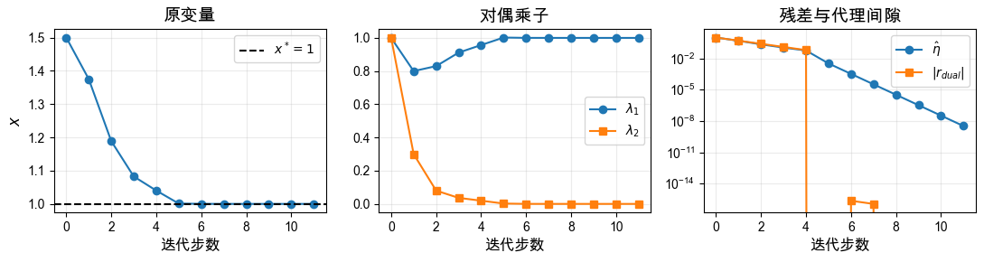
观察结果：

$x$ 从严格可行点 1.5 逐渐靠近边界最优解 $x^\star=1$ ，但每一步仍保持 $x>1$ 。
最优点处第一个约束 $1-x\le0$ 是活跃约束，因此 $\lambda_1$ 靠近 1；第二个约束 $x-2\le0$ 不活跃，因此 $\lambda_2$ 靠近 0。
代理对偶间隙 $\hat\eta$ 持续下降，说明扰动 KKT 条件逐渐接近原问题的 KKT 条件。

100维线性规划例子¶

现在看一个稍大的盒约束线性规划：

\begin{array}{ll} \text{minimize} & c^T x \\ \text{subject to} & 0\le x_i\le 1,\quad i=1,\ldots,100. \end{array}

(10)

这里取 $c_i>0$ ，因此最优解是 $x^\star=0$ ，最优值是 0。为了使用原对偶内点法，把不等式写成

-x_i\le 0,\qquad x_i-1\le 0.

(11)

所以这个例子有 $n=100$ 个变量和 $m=200$ 个不等式约束。

np.random.seed(7)

n_large = 100
c_large = 0.5 + np.random.rand(n_large)
D_large = np.vstack([-np.eye(n_large), np.eye(n_large)])
m_large = 2 * n_large

def lp100_constraints(x):
    return np.concatenate([-x, x - 1.0])

def lp100_objective(x):
    return c_large @ x

def lp100_residual(x, lam, t):
    r_dual = c_large + D_large.T @ lam
    r_cent = -lam * lp100_constraints(x) - np.ones(m_large) / t
    return np.concatenate([r_dual, r_cent])

def lp100_surrogate_gap(x, lam):
    return -lp100_constraints(x) @ lam

def lp100_is_strictly_feasible(x, lam):
    return np.all(lp100_constraints(x) < 0) and np.all(lam > 0)

def lp100_direction(x, lam, t):
    f = lp100_constraints(x)
    residual_value = lp100_residual(x, lam, t)
    jacobian = np.block([
        [np.zeros((n_large, n_large)), D_large.T],
        [-np.diag(lam) @ D_large, -np.diag(f)],
    ])
    step = np.linalg.solve(jacobian, -residual_value)
    return step[:n_large], step[n_large:]

x_large = 0.5 * np.ones(n_large)
lam_large = np.ones(m_large)
history_large = []

start_time = time.perf_counter()

for k in range(max_iter):
    eta = lp100_surrogate_gap(x_large, lam_large)
    r_dual_norm = np.linalg.norm(c_large + D_large.T @ lam_large)
    history_large.append([
        k,
        lp100_objective(x_large),
        eta,
        r_dual_norm,
        np.linalg.norm(x_large),
    ])

    if eta <= eps and r_dual_norm <= eps_feas:
        break

    t = mu * m_large / eta
    dx, dlam = lp100_direction(x_large, lam_large, t)
    residual_norm = np.linalg.norm(lp100_residual(x_large, lam_large, t))

    step_size = 1.0
    while not lp100_is_strictly_feasible(
        x_large + step_size * dx,
        lam_large + step_size * dlam,
    ):
        step_size *= beta

    while (
        np.linalg.norm(
            lp100_residual(
                x_large + step_size * dx,
                lam_large + step_size * dlam,
                t,
            )
        )
        > (1.0 - alpha * step_size) * residual_norm
    ):
        step_size *= beta

    x_large = x_large + step_size * dx
    lam_large = lam_large + step_size * dlam

runtime = time.perf_counter() - start_time
history_large = np.array(history_large)

print_large(f"维度 n = {n_large}, 不等式约束个数 m = {m_large}")
print_large(f"迭代步数 = {len(history_large) - 1}")
print_large(f"运行时间 = {runtime * 1000:.2f} ms")
print_large(f"最终目标函数值 = {lp100_objective(x_large):.3e}")
print_large(f"最终代理对偶间隙 = {lp100_surrogate_gap(x_large, lam_large):.3e}")
print_large(f"最终 dual residual = {np.linalg.norm(c_large + D_large.T @ lam_large):.3e}")

plt.figure(figsize=(10, 3.4))

plt.subplot(1, 2, 1)
plt.plot(history_large[:, 0], history_large[:, 1], "o-", label=r"$c^T x$")
plt.plot(history_large[:, 0], history_large[:, 4], "s-", label=r"$\|x\|_2$")
plt.yscale("log")
plt.xlabel("迭代步数", fontsize=12)
plt.title("原变量靠近最优解", fontsize=14)
plt.grid(alpha=0.25)
plt.legend()

plt.subplot(1, 2, 2)
plt.plot(history_large[:, 0], history_large[:, 2], "o-", label=r"$\hat\eta$")
plt.plot(history_large[:, 0], history_large[:, 3], "s-", label=r"$\|r_{dual}\|_2$")
plt.yscale("log")
plt.xlabel("迭代步数", fontsize=12)
plt.title("残差与代理间隙", fontsize=14)
plt.grid(alpha=0.25)
plt.legend()

plt.tight_layout()
plt.show()

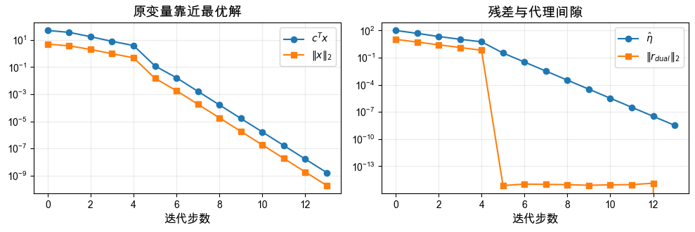
观察结果：

这个 100 维例子仍然使用同一套原对偶残差和牛顿线性化，只是把一维变量换成了向量。
因为所有 $c_i>0$ ，最优解在下边界 $x_i=0$ 上，图中 $\|x\|_2$ 和目标函数值都逐步下降。
运行时间包含每一步构造并求解一个 $300\times 300$ 的线性方程组。

总结¶

这个 notebook 用一个一维例子和一个 100 维 LP 例子展示了原对偶内点法的核心结构：

用 $r_{\mathrm{dual}}$ 检查驻点条件；
用 $r_{\mathrm{cent}}$ 检查扰动互补关系；
通过牛顿系统同时更新 $x$ 和 $\lambda$ ；
用线搜索保持严格可行性与正乘子；
在较高维例子中，可以用运行时间观察线性方程组求解带来的计算成本。