7.1 障碍方法 - MATH3806 Code

这个 notebook 与第7章第1部分“障碍方法”对应，重点观察：

对数障碍函数如何把不等式约束变成光滑惩罚项；
中心点 $x^\star(t)$ 如何随障碍参数 $t$ 增大而靠近原问题最优解；
误差界 $0\le f_0(x^\star(t))-p^\star\le m/t$ 在一个二维线性规划例子中的表现；
障碍方法如何通过外层更新 $t\leftarrow \mu t$ 逐步提高精度。

学习目标¶

完成本 notebook 后，希望能够：

画出 $-\frac{1}{t}\log(-u)$ 并解释它为什么只允许严格可行点；
用 cvxpy 写出并求解障碍子问题；
通过数值图像验证中心路径和误差界 $m/t$ ；
用一个简单的外层迭代演示障碍方法。

import numpy as np
import matplotlib.pyplot as plt

import cvxpy as cp
from IPython.display import HTML, display

plt.rcParams["font.sans-serif"] = [
    "Arial Unicode MS",
    "PingFang SC",
    "Heiti TC",
    "Microsoft YaHei",
    "SimHei",
]
plt.rcParams["axes.unicode_minus"] = False


def print_large(text):
    display(HTML(f'<font size="3">{text}</font>'))

1. 对数障碍函数的形状¶

对约束 $u=f_i(x)\le 0$ ，原本可以用指示函数

I_-(u)=\begin{cases} 0, & u\le 0,\\ \infty, & u>0 \end{cases}

(1)

表示“不满足约束就不允许”。为了使用梯度法或牛顿法，我们改用光滑近似

\widehat I_-(u)=-\frac{1}{t}\log(-u), \qquad u<0.

(2)

它在边界 $u=0$ 附近会迅速增大，因此会把迭代点留在严格可行域内部。

u_grid = np.linspace(-3.0, -1.0e-3, 1000)

plt.figure(figsize=(4, 2.5))
colors = ["#e11d48", "#d97706", "#0f766e", "#2563eb"]
for t, color in zip([0.5, 1.0, 2.0, 5.0], colors):
    plt.plot(u_grid, -np.log(-u_grid) / t, color=color, linewidth=2,
             label=rf"$t={t:g}$")

plt.axhline(0, color="#475569", linestyle="--", linewidth=1)
plt.axvline(0, color="#475569", linestyle="--", linewidth=1)
plt.xlim([-3, 0.5])
plt.ylim([-1, 12])
plt.xlabel(r"$u=f_i(x)$", size=12)
plt.ylabel(r"$-\log(-u)/t$", size=12)
plt.title("对数障碍函数", size=14)
plt.legend(loc="upper left", ncol=2, fontsize=12, frameon=True)
plt.grid(alpha=0.25)
plt.tight_layout()
plt.show()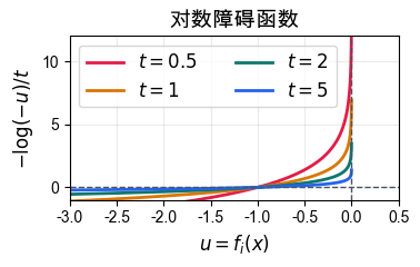

观察结果：

对数障碍只在 $u<0$ 上有定义，所以算法天然会在严格可行域内部工作。
越靠近边界 $u=0$ ，函数值越大，相当于给边界附近加上一堵“软墙”。
当 $t$ 变大时， $-\log(-u)/t$ 的整体高度变低，因此障碍子问题会更接近原问题。

2. 二维线性规划例子¶

考虑如下二维线性规划例子。原问题为

\begin{array}{ll} \text{minimize} & 8x+5y \\ \text{subject to} & x+y=1,\\ & 60x+40y\ge 50,\\ & 20x+10y\ge 15,\\ & x\ge 0,\\ & x\le 1. \end{array}

(3)

由 $x+y=1$ 可知目标函数为 $8x+5(1-x)=3x+5$ 。前两个不等式都要求 $x\ge 0.5$ ，所以原问题的最优解为

(x^\star,y^\star)=(0.5,0.5),\qquad p^\star=6.5.

(4)

这里共有 $m=4$ 个不等式约束，因此理论误差界是 $m/t=4/t$ 。

c = np.array([8.0, 5.0])
A = np.array([[1.0, 1.0]])
b = np.array([1.0])
z_star = np.array([0.5, 0.5])
p_star = c @ z_star
m = 4


def objective_value(z):
    return c @ z


def margins(z):
    # Positive margins h_i(z); constraints are h_i(z) >= 0.
    x, y = z
    return np.array([
        60.0 * x + 40.0 * y - 50.0,
        20.0 * x + 10.0 * y - 15.0,
        x,
        1.0 - x,
    ])


def solve_barrier_subproblem(t, z_start=None):
    z = cp.Variable(2)
    if z_start is not None:
        z.value = z_start

    x, y = z[0], z[1]
    h = cp.hstack([
        60.0 * x + 40.0 * y - 50.0,
        20.0 * x + 10.0 * y - 15.0,
        x,
        1.0 - x,
    ])
    objective = cp.Minimize(t * c @ z - cp.sum(cp.log(h)))
    problem = cp.Problem(objective, [A @ z == b])

    try:
        problem.solve(solver=cp.CLARABEL, warm_start=True)
    except cp.SolverError:
        problem.solve(warm_start=True)

    if problem.status not in [cp.OPTIMAL, cp.OPTIMAL_INACCURATE] or z.value is None:
        raise RuntimeError(f"Barrier subproblem failed for t={t}: {problem.status}")

    z_value = np.asarray(z.value, dtype=float)
    return z_value, objective_value(z_value)

3. 计算中心路径¶

对每个 $t$ ，我们求解障碍子问题

\begin{array}{ll} \text{minimize} & t(8x+5y)-\log(60x+40y-50)-\log(20x+10y-15) \\ &\qquad\qquad -\log x-\log(1-x)\\ \text{subject to} & x+y=1. \end{array}

(5)

注意：这里的 $t$ 是障碍参数，不是回溯线搜索中的步长。

mu = 3
t_list = mu ** np.arange(0, 12)
center_points = np.zeros((len(t_list), 2))
objective_values = np.zeros(len(t_list))

for i, t in enumerate(t_list):
    center_points[i], objective_values[i] = solve_barrier_subproblem(float(t))

objective_gaps = objective_values - p_star
if np.min(objective_gaps) < -1.0e-8:
    raise RuntimeError("Objective gap should be nonnegative; check solver accuracy.")

gap_bound = m / t_list
coordinate_errors = np.abs(center_points - z_star)

print_large(f"共求解 {len(t_list)} 个障碍子问题")
print_large(f"第一个中心点 = {np.round(center_points[0], 6)}")
print_large(f"最后一个中心点 = {np.round(center_points[-1], 6)}")
print_large(f"最后一个目标函数误差 = {objective_gaps[-1]:.3e}")

plt.figure(figsize=(9.6, 2.8))

plt.subplot(1, 3, 1)
plt.plot(t_list, objective_gaps, "o-", color="#2563eb",
         linewidth=2, markersize=5, label="数值误差")
plt.plot(t_list, gap_bound, "--", color="#e11d48",
         linewidth=2, label=r"理论上界 $m/t$")
plt.xscale("log")
plt.yscale("log")
plt.xlabel(r"$t$", size=12)
plt.ylabel("误差", size=12)
plt.title("目标函数误差", size=14)
plt.grid(alpha=0.25, which="both")
plt.legend(loc="lower left", fontsize=12, frameon=True)

plt.subplot(1, 3, 2)
plt.plot(t_list, coordinate_errors[:, 0], "o-", color="#0f766e",
         linewidth=2, markersize=5, label=r"$|x(t)-0.5|$")
plt.plot(t_list, coordinate_errors[:, 1], "s--", color="#d97706",
         linewidth=2, markersize=5, label=r"$|y(t)-0.5|$")
plt.xscale("log")
plt.yscale("log")
plt.xlabel(r"$t$", size=12)
plt.ylabel("误差", size=12)
plt.title("坐标误差", size=14)
plt.grid(alpha=0.25, which="both")
plt.legend(loc="lower left", fontsize=12, frameon=True)

plt.subplot(1, 3, 3)
plt.plot(center_points[:, 0], center_points[:, 1], "o-", color="#0f766e",
         linewidth=2, markersize=5, label="中心路径")
plt.scatter(z_star[0], z_star[1], marker="*", s=150, color="#e11d48",
            edgecolor="white", linewidth=0.8, zorder=5, label="原最优解")
plt.xlim(0.47, 0.82)
plt.ylim(0.18, 0.53)
plt.gca().set_aspect("equal", adjustable="box")
plt.xlabel(r"$x$", size=12)
plt.ylabel(r"$y$", size=12)
plt.title("中心路径", size=14)
plt.grid(alpha=0.25)
plt.legend(loc="lower left", fontsize=12, frameon=True)

plt.tight_layout()
plt.show()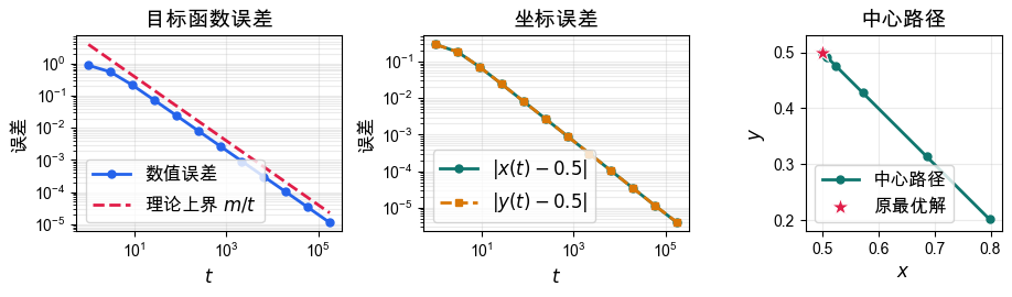

观察结果：

随着 $t$ 增大，中心点沿着严格可行域内部靠近 $(0.5,0.5)$ 。
目标函数误差始终低于理论界 $m/t$ 。
坐标误差也随 $t$ 增大而下降，但理论界直接控制的是目标函数值误差。

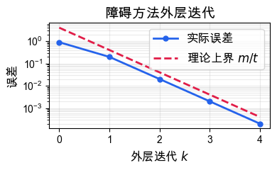
4. 障碍方法的外层迭代¶

现在把中心路径真正串起来：从一个严格可行点出发，求当前 $t$ 下的中心点；然后把这个中心点作为下一轮的初始点，并令 $t\leftarrow\mu t$ 。

这里仍然直接处理二维变量 $(x,y)$ ，并用 cvxpy 求解每个障碍子问题。外层迭代只保留最关键的信息：中心点、实际误差和理论上界 $m/t$ 。

t = 1.0
mu_path = 10.0
epsilon = 1.0e-3
z_start = np.array([0.75, 0.25])
barrier_history = []

while True:
    z_center, objective_at_center = solve_barrier_subproblem(t, z_start)
    gap = objective_at_center - p_star
    bound = m / t
    barrier_history.append([
        len(barrier_history), t, z_center[0], z_center[1], gap, bound,
    ])

    if bound <= epsilon:
        break

    z_start = z_center
    t *= mu_path

barrier_history = np.array(barrier_history, dtype=float)

print(" k       t        x(t)      y(t)      gap       m/t")
for row in barrier_history:
    print(
        f"{int(row[0]):2d}  {row[1]:8.0f}  {row[2]:8.5f}  "
        f"{row[3]:8.5f}  {row[4]:8.2e}  {row[5]:8.2e}"
    )

plt.figure(figsize=(4, 2.5))
plt.semilogy(barrier_history[:, 0], barrier_history[:, 4], "o-",
             color="#2563eb", linewidth=2, markersize=5, label="实际误差")
plt.semilogy(barrier_history[:, 0], barrier_history[:, 5], "--",
             color="#e11d48", linewidth=2, label=r"理论上界 $m/t$")
plt.xlabel("外层迭代 $k$", size=12)
plt.ylabel("误差", size=12)
plt.title("障碍方法外层迭代", size=14)
plt.grid(alpha=0.25, which="both")
plt.legend(fontsize=12, frameon=True)
plt.tight_layout()
plt.show()

 k       t        x(t)      y(t)      gap       m/t
 0         1   0.79829   0.20171  8.95e-01  4.00e+00
 1        10   0.56550   0.43450  1.97e-01  4.00e-01
 2       100   0.50667   0.49333  2.00e-02  4.00e-02
 3      1000   0.50067   0.49933  2.00e-03  4.00e-03
 4     10000   0.50007   0.49993  2.00e-04  4.00e-04

总结¶

这个 notebook 验证或强调了四件事：

对数障碍函数把边界变成光滑但非常陡峭的惩罚项，因此迭代点留在严格可行域内部。
中心点 $x^\star(t)$ 随 $t$ 增大逐渐靠近原问题的最优解。
目标函数误差满足 $0\le f_0(x^\star(t))-p^\star\le m/t$ ，二维例子中的数值结果与理论一致。
障碍方法通过逐步增大 $t$ ，用一串较容易求解的子问题逼近原问题。