4.2 Logistic 回归

目标：用一个二维二分类例子说明 Logistic 回归如何转化为凸优化问题。

主线：生成数据、写出 cvxpy 优化问题、画出分类边界，最后用 sklearn 做一个简短对照。

import numpy as np
import matplotlib.pyplot as plt

import cvxpy as cp

from sklearn.datasets import make_classification
from sklearn.linear_model import LogisticRegression
from sklearn.model_selection import train_test_split

import matplotlib.pyplot as plt
plt.rcParams["font.sans-serif"] = ["Arial Unicode MS", "PingFang SC", "Heiti TC", "Microsoft YaHei", "SimHei"]
plt.rcParams["axes.unicode_minus"] = False

seed = 42
num_samples = 500
reg_strength = 1.0e-2

1. 创建二维分类数据¶

X, y = make_classification(
    n_samples=num_samples,
    n_features=2,
    n_informative=2,
    n_redundant=0,
    n_clusters_per_class=1, 
    class_sep=1.4, # increase class separation for better visualization
    flip_y=0.06, # flip 6% of the labels to introduce noise
    random_state=seed,
)

X_train, X_test, y_train, y_test = train_test_split(
    X,
    y,
    test_size=0.25,
    random_state=seed,
    stratify=y,
)

print(f"训练集大小: {X_train.shape}")
print(f"测试集大小: {X_test.shape}")
print(f"测试集中类别 1 的比例: {np.mean(y_test == 1):.2f}")

训练集大小: (375, 2)
测试集大小: (125, 2)
测试集中类别 1 的比例: 0.51

plt.figure(figsize=(5, 4))
plt.scatter(
    X_train[y_train == 0, 0],
    X_train[y_train == 0, 1],
    label="class 0",
    alpha=0.75,
)
plt.scatter(
    X_train[y_train == 1, 0],
    X_train[y_train == 1, 1],
    label="class 1",
    alpha=0.75,
)
plt.xlabel("$x_1$", size=12)
plt.ylabel("$x_2$", size=12)
plt.title("训练数据", size=14)
plt.legend()
plt.tight_layout()
plt.show()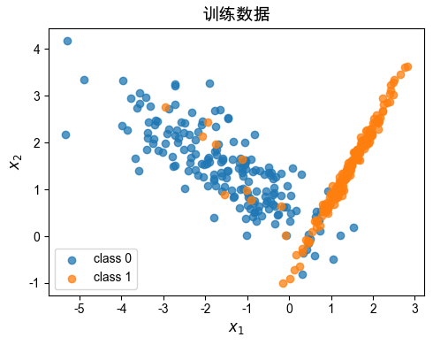

2. 用 `cvxpy` 求解 Logistic 回归¶

记 $s_i=a^T x_i+b$ 。带 $L2$ 正则化的目标函数为

\sum_i \left(\log(1+e^{s_i})-y_i s_i\right) +\frac{\lambda}{2}\|a\|_2^2.

(1)

第一项是负对数似然，第二项用于控制参数大小。

num_features = X_train.shape[1]
a = cp.Variable(num_features)
b = cp.Variable()

s = X_train @ a + b
negative_log_likelihood = cp.sum(
    cp.logistic(s) - cp.multiply(y_train, s)
)
regularization = 0.5 * reg_strength * cp.sum_squares(a)

objective = cp.Minimize(negative_log_likelihood + regularization)
problem = cp.Problem(objective)
problem.solve()

print(f"求解状态: {problem.status}")
print(f"a = {np.round(a.value, 3)}")
print(f"b = {b.value:.3f}")

求解状态: optimal
a = [2.077 0.593]
b = -0.804

test_scores = X_test @ a.value + b.value
y_pred = (test_scores >= 0).astype(int)
accuracy = np.mean(y_pred == y_test)

print(f"测试集准确率: {accuracy:.3f}")

测试集准确率: 0.872

x1_min, x1_max = X[:, 0].min() - 0.5, X[:, 0].max() + 0.5
x2_min, x2_max = X[:, 1].min() - 0.5, X[:, 1].max() + 0.5

grid_x1, grid_x2 = np.meshgrid(
    np.linspace(x1_min, x1_max, 120),
    np.linspace(x2_min, x2_max, 120),
)
grid_points = np.c_[grid_x1.ravel(), grid_x2.ravel()]
grid_scores = grid_points @ a.value + b.value
grid_scores = grid_scores.reshape(grid_x1.shape)

plt.figure(figsize=(5, 4))
plt.contourf(
    grid_x1,
    grid_x2,
    grid_scores >= 0,
    levels=[-0.5, 0.5, 1.5],
    alpha=0.18,
)
plt.contour(
    grid_x1,
    grid_x2,
    grid_scores,
    levels=[0],
    colors="black",
    linewidths=2,
)
plt.scatter(
    X_test[y_test == 0, 0],
    X_test[y_test == 0, 1],
    label="class 0",
    alpha=0.85,
)
plt.scatter(
    X_test[y_test == 1, 0],
    X_test[y_test == 1, 1],
    label="class 1",
    alpha=0.85,
)
plt.xlabel("$x_1$", size=12)
plt.ylabel("$x_2$", size=12)
plt.title(f"决策边界，准确率 = {accuracy:.3f}", size=14)
plt.legend()
plt.tight_layout()
plt.show()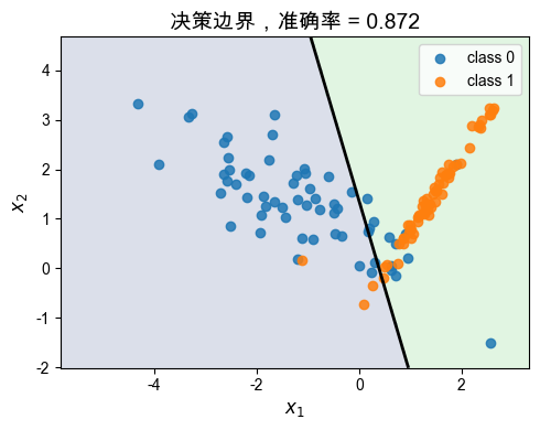

3. 可选：与 `sklearn` 做对照¶

sklearn 是常用机器学习工具之一。这里仅用于检查结果是否一致。

sk_model = LogisticRegression(
    C=1 / reg_strength, # sklearn 中的正则化强度参数是 C 的倒数
    penalty="l2", 
    solver="lbfgs", # 默认的优化算法，适用于小型数据集
    max_iter=1000,
)
sk_model.fit(X_train, y_train)
sk_accuracy = sk_model.score(X_test, y_test)

print(f"cvxpy 准确率:   {accuracy:.3f}")
print(f"sklearn 准确率: {sk_accuracy:.3f}")
print(f"cvxpy 的 a:   {np.round(a.value, 3)}")
print(f"sklearn 的 a: {np.round(sk_model.coef_[0], 3)}")

cvxpy 准确率:   0.872
sklearn 准确率: 0.872
cvxpy 的 a:   [2.077 0.593]
sklearn 的 a: [2.077 0.594]

1. 创建二维分类数据¶

2. 用 cvxpy 求解 Logistic 回归¶

3. 可选：与 sklearn 做对照¶

2. 用 `cvxpy` 求解 Logistic 回归¶

3. 可选：与 `sklearn` 做对照¶