2.3 二次规划
二次规划是凸优化中非常重要且常见的一类问题。它典型的特点是目标函数是关于变量的二次函数,而所有的约束条件均为线性模型(包括等式和不等式限制)。这类问题被广泛应用于诸如回归分析、数据分类、支持向量机以及金融量化中的投资组合优化等各类生产生活场景。
本节目标
我们将通过以下 3 个典型案例,介绍如何用 Python / CVXPY 的语法来解决二次规划类优化模型:
最小二乘问题(无约束):通过最小化真实数据和模型误差的平方和,来拟合极佳估计参数。
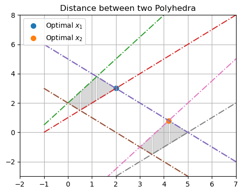
多面体间的最小距离:计算多维空间中,在由多组不等式定义的复杂多面体之间寻找最邻近点的最短欧几里得距离。
Markowitz 投资组合优化:在金融中经典的均值-方差模型。如何在保证所期望资金收益下界的严格前提下,智能分配多元资产以追求最小化投资受损的全局风险(方差)。
注:
此处的展示数据偏向基础并生成随机种子,仅作为直观的理论模型教学演示之用,实际场景要考虑更多的要素。
对于如何使用SciPy求解同样的问题,将作为作业。
import cvxpy as cp
import numpy as np
import matplotlib.pyplot as plt
例子1:最小二乘
# 作业1的第一题的最小二乘问题
A = np.transpose(np.vstack((np.ones(5), [0, 5, 10, 15, 20])))
b = np.transpose(np.array([0, 1.27, 2.16, 2.86, 3.44]))

# 解析解
c = np.linalg.solve(A.T @ A, A.T @ b)
print("解析解 = [{:.4f}, {:.4f}]\n".format(c[0], c[1]))

# 创建优化变量
x = cp.Variable(2)

# 创建目标函数
obj = cp.Minimize(cp.sum_squares(A @ x - b))

# 创建优化问题
prob = cp.Problem(obj)
prob.solve()

# 输出结果
print("求解状态:", prob.status)
print("最优值:", f"{prob.value:.4f}" if prob.value is not None else None)
print("最优变量 x:", np.round(x.value, 4) if x.value is not None else None)
解析解 = [0.2520, 0.1694]
求解状态: optimal
最优值: 0.1830
最优变量 x: [0.252 0.1694]
例子2:多面体间的距离
a1 = np.array([1,1])
b1 = 5
a2 = np.array([-1,-1])
b2 = -2
a3 = np.array([-1.5,1])
b3 = 2
a4 = np.array([1,-1])
b4 = -1

A1 = np.vstack((a1,a2,a3,a4))
b1 = np.array([b1,b2,b3,b4])

def plot_Polyhedra(A1, b1, A2, b2, cx, cy):
    x_grid = np.linspace(-1, 10, 200)
    y_list = []
    for i in range(4):
        a = A1[i,:]
        y_grid = (b1[i] - a[0] * x_grid)/a[1]
        y_list.append(y_grid)
        plt.plot(x_grid, y_grid, '-.')

    y1, y2, y3, y4 = y_list
    # Fill the region between the lines
    plt.fill_between(x_grid, y2, y3, where= (y2 < y3) & (y4 < y2), color='gray',alpha=0.3)
    plt.fill_between(x_grid, y4, y3, where= (y4 < y3) & (y3 < y1) & (y2 < y4), color='gray',alpha=0.3)
    plt.fill_between(x_grid, y4, y1, where= (y4 < y1) & (y1 < y3), color='gray',alpha=0.3)

    y_list = []
    for i in range(4):
        a = A2[i,:]
        y_grid = (b2[i] - a[0] * x_grid)/a[1]
        y_list.append(y_grid)
        plt.plot(x_grid, y_grid, '-.')

    y1, y2, y3, y4 = y_list
    # Fill the region between the lines
    plt.fill_between(x_grid, y2, y3, where= (y2 < y3) & (y4 < y2), color='gray',alpha=0.3)
    plt.fill_between(x_grid, y4, y3, where= (y4 < y3) & (y3 < y1) & (y2 < y4), color='gray',alpha=0.3)
    plt.fill_between(x_grid, y4, y1, where= (y4 < y1) & (y1 < y3), color='gray',alpha=0.3)

    plt.ylim([0 - np.abs(cy), 5 + np.abs(cy)])
    plt.xlim([1 - np.abs(cx), 4 + np.abs(cx)])

    plt.grid(True)
# 设定问题

# 平移
cx = 3
cy = 4

A2 = A1
b2 = b1 + A1[:,0] * cx + A1[:,1] * cy

fig = plt.figure(figsize=(5,4))
plot_Polyhedra(A1, b1, A2, b2, cx, cy)
plt.tight_layout()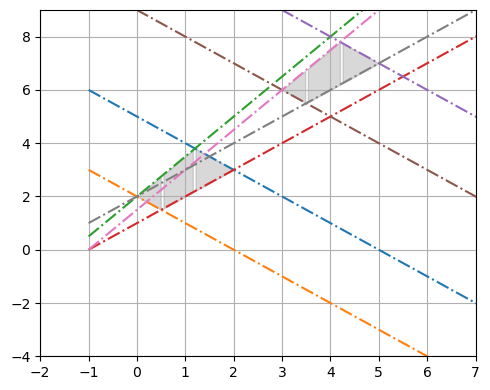
# 创建优化变量
x1 = cp.Variable(2)
x2 = cp.Variable(2)
# 创建限制条件
constraints = [A1 @ x1 <= b1, A2 @ x2 <= b2]
# 创建目标函数
obj = cp.Minimize(cp.sum_squares(x1 - x2))
# 创建优化问题
prob = cp.Problem(obj, constraints)
prob.solve()
# 输出结果
print("求解状态:", prob.status)
print("最优距离:", f"{np.sqrt(prob.value):.4f}" if prob.value is not None else None)
print("最优变量 x1:", np.round(x1.value, 4) if x1.value is not None else None)
print("最优变量 x2:", np.round(x2.value, 4) if x2.value is not None else None)
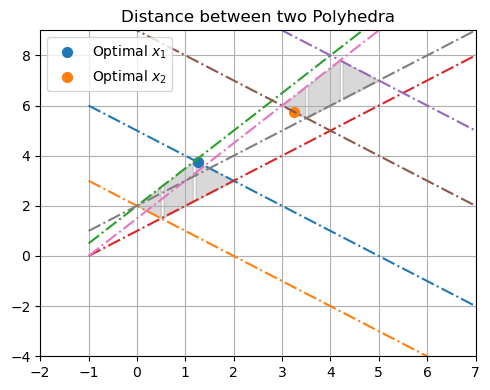
fig = plt.figure(figsize=(5,4))
plot_Polyhedra(A1, b1, A2, b2, cx, cy)
if x1.value is not None and x2.value is not None:
plt.scatter(x1.value[0], x1.value[1], s=50, label=r"Optimal $x_1$")
plt.scatter(x2.value[0], x2.value[1], s=50, label=r"Optimal $x_2$")
plt.legend(loc="upper left")
plt.title("Distance between two Polyhedra")
plt.tight_layout()
plt.show()求解状态: optimal
最优距离: 2.8284
最优变量 x1: [1.2537 3.7463]
最优变量 x2: [3.2537 5.7463]
# 设定问题

# 平移
cx = 3
cy = -3

A2 = A1
b2 = b1 + A1[:,0] * cx + A1[:,1] * cy

fig = plt.figure(figsize=(5,4))
plot_Polyhedra(A1, b1, A2, b2, cx, cy)
plt.tight_layout()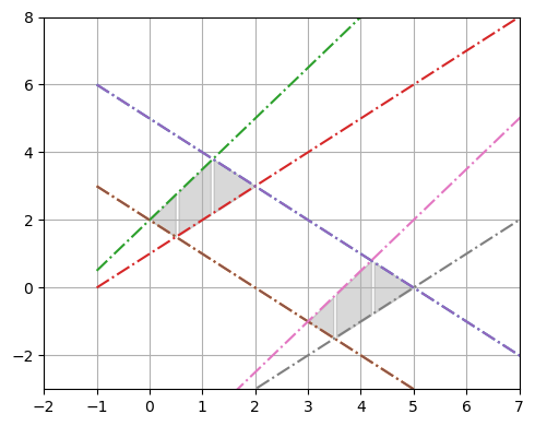
# 创建优化变量
x1 = cp.Variable(2)
x2 = cp.Variable(2)

# 创建限制条件
constraints = [A1 @ x1 <= b1, A2 @ x2 <= b2]

# 创建目标函数
obj = cp.Minimize(cp.sum_squares(x1 - x2))

# 创建优化问题
prob = cp.Problem(obj, constraints)
prob.solve()

# 输出结果
print("求解状态:", prob.status)
print("最优距离:", f"{np.sqrt(prob.value):.4f}" if prob.value is not None else None)
print("最优变量 x1:", np.round(x1.value, 4) if x1.value is not None else None)
print("最优变量 x2:", np.round(x2.value, 4) if x2.value is not None else None)

fig = plt.figure(figsize=(5,4))
plot_Polyhedra(A1, b1, A2, b2, cx, cy)
if x1.value is not None and x2.value is not None:
    plt.scatter(x1.value[0], x1.value[1], s=50, label=r"Optimal $x_1$")
    plt.scatter(x2.value[0], x2.value[1], s=50, label=r"Optimal $x_2$")
plt.legend(loc="upper left")
plt.title("Distance between two Polyhedra")
plt.tight_layout()
plt.show()
求解状态: optimal
最优距离: 3.1113
最优变量 x1: [2. 3.]
最优变量 x2: [4.2 0.8]
例子3:Markowitz 投资组合优化
# 设定问题
np.random.seed(1)  # 为可复现结果

n = 10
pbar = np.random.rand(n) - 0.3
A = 0.05 * np.random.randn(n, n)
Σ = A.T @ A
rmin = 0.1

def solve_Markowitz_problem(n, pbar, Σ, rmin, verbose=False):
    # 创建优化变量
    # 此处我们考虑不允许做空
    x = cp.Variable(n, nonneg=True)

    # 创建限制条件
    constraints = [pbar @ x >= rmin, np.ones(n) @ x == 1]

    # 创建目标函数
    obj = cp.Minimize(cp.quad_form(x, Σ))

    # 创建优化问题
    prob = cp.Problem(obj, constraints)
    prob.solve()

    if verbose:
        print("求解状态:", prob.status)
        print("最优值:", f"{prob.value:.4f}" if prob.value is not None else None)
        print("最优变量 x:", np.round(x.value, 4) if x.value is not None else None)

    if prob.status not in {cp.OPTIMAL, cp.OPTIMAL_INACCURATE}:
        return None, prob

    return x.value, prob
plt.figure(figsize=(5,3))
plt.plot(pbar, 'x', label=r"$\bar{p}_i$")
plt.plot(pbar + np.sqrt(np.diag(Σ)), label=r"$\bar{p}_i + σ_i$")
plt.plot(pbar - np.sqrt(np.diag(Σ)), label=r"$\bar{p}_i - σ_i$")
for rmin in [0.1, 0.3]:
x_opt, prob = solve_Markowitz_problem(n, pbar, Σ, rmin, verbose=True)
if x_opt is not None:
plt.plot(x_opt, 'o-.', label=r"$x_i$ for $r_\min$ = {:.1f}".format(rmin))
else:
print(f"r_min = {rmin:.1f} 时问题不可行。")
print()
plt.tight_layout()
plt.legend(bbox_to_anchor=(1, 0.8))
plt.grid(True)
plt.show()求解状态: optimal
最优值: 0.0005
最优变量 x: [0.2116 0. 0.086 0.0281 0. 0. 0.0198 0.2 0.1019 0.3527]
求解状态: optimal
最优值: 0.0070
最优变量 x: [0.0435 0.4594 0. 0. 0. 0. 0. 0. 0.1189 0.3782]
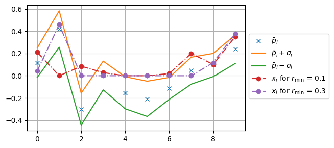
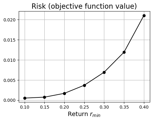
下面实验的含义:需要高回报的情况,我们需要在更小的范围的可行解中进行优化,因此最优的函数值(随机性)更高
rmin_list = np.arange(0.1, 0.5, 0.05)
risk_list = np.full(len(rmin_list), np.nan)
for j, rmin in enumerate(rmin_list):
    _, prob = solve_Markowitz_problem(n, pbar, Σ, rmin)
    if prob.status in {cp.OPTIMAL, cp.OPTIMAL_INACCURATE}:
        risk_list[j] = prob.value

plt.figure(figsize=(5,4))
plt.plot(rmin_list, risk_list, 'k-o')
plt.xlabel(r'Return $r_{min}$', fontsize=14)
plt.title('Risk (objective function value)', fontsize=16)
plt.tight_layout()
plt.grid(True)
plt.show()