3.2 牛顿法

这个 notebook 与第3章第3部分的课件对应，重点观察：

牛顿法如何利用二阶信息产生方向
阻尼牛顿法与纯牛顿阶段的区别
为什么牛顿法在极小值点附近通常比梯度下降更快

学习目标¶

完成本 notebook 后，希望能够：

写出牛顿步 $\Delta x = -\big(\nabla^2 f(x)\big)^{-1}\nabla f(x)$
观察阻尼牛顿法的步长何时会变成 $t=1$
用数值结果对比梯度法与牛顿法的收敛速度
在图像中识别局部二次收敛的迹象

在开始前，可以先思考两个问题：

对二次函数来说，如果我们已经知道曲率矩阵 $Q$ ，为什么用 $Q^{-1}$ 来缩放梯度可能更合理？
在梯度下降法里，为什么条件数大时会出现之字形轨迹？

import os
import time

import matplotlib.pyplot as plt
import numpy as np
from IPython.display import HTML, display

os.makedirs('assets', exist_ok=True)

plt.rcParams['font.sans-serif'] = ['Arial Unicode MS', 'PingFang SC', 'Heiti TC', 'SimHei']
plt.rcParams['axes.unicode_minus'] = False

print_large = lambda text: display(HTML(f'<font size="3">{text}</font>'))

class Problem:
    def __init__(self, dim=2, alpha=0.1, beta=0.8, f=None, df=None, hessian=None):
        self.dim = dim
        self.alpha = alpha
        self.beta = beta
        self.tol = 1.0e-8
        self.ref_state = None
        self.condition = 'grad'
        self.P = np.eye(dim)
        self.method = 'gradient' # gradient or newton
        self.f = f
        self.df = df
        self.hessian = hessian

    def backtracking_line_search(self, x, d):
        t = 1.0
        k = 0
        fx = self.f(x)
        directional_derivative = np.dot(self.df(x), d)

        while self.f(x + t * d) > fx + self.alpha * t * directional_derivative:
            t *= self.beta
            k += 1
        return t, k

    def gradient_propose(self, x):
        if self.method == 'gradient':
            matrix = self.P
        elif self.method == 'newton':
            matrix = self.hessian(x)
        else:
            raise ValueError('method must be gradient or newton')
        return -np.linalg.solve(matrix, self.df(x))

    def newton_decrement(self, x):
        hess = self.hessian(x)
        grad = self.df(x)
        return np.sqrt(grad @ np.linalg.solve(hess, grad))

    def stop_condition(self, x):
        if self.condition == 'ref_state':
            return np.linalg.norm(x - self.ref_state) < self.tol
        if self.condition == 'grad':
            return np.linalg.norm(self.df(x)) < self.tol
        if self.condition == 'newton_decrement':
            return self.newton_decrement(x) ** 2 / 2 <= self.tol
        raise ValueError('unknown stopping condition')

    def solve(self, x0, max_iter=100):
        t_begin = time.time()

        x = x0.astype(float).copy()
        trajectory = [x.copy()]
        t_list = []
        decrement_list = []

        for _ in range(max_iter):
            if self.method == 'newton':
                decrement_list.append(self.newton_decrement(x))
            d = self.gradient_propose(x)
            t, _ = self.backtracking_line_search(x, d)
            x = x + t * d
            t_list.append(t)
            trajectory.append(x.copy())
            if self.stop_condition(x):
                break

        if self.method == 'newton':
            decrement_list.append(self.newton_decrement(x))

        runtime = time.time() - t_begin
        return np.array(trajectory), runtime, t_list, decrement_list

    def plot_contour(self, xmin, xmax, ymin, ymax):
        grid_x = np.linspace(xmin, xmax, 400)
        grid_y = np.linspace(ymin, ymax, 300)
        grid_X, grid_Y = np.meshgrid(grid_x, grid_y)
        Z = np.zeros_like(grid_X)

        for i in range(grid_X.shape[0]):
            for j in range(grid_X.shape[1]):
                Z[i, j] = self.f(np.array([grid_X[i, j], grid_Y[i, j]]))

        contour = plt.contourf(grid_X, grid_Y, Z, levels=20, cmap='Blues')
        plt.colorbar(contour)
        plt.xlabel(r'$x_1$', fontsize=12)
        plt.ylabel(r'$x_2$', fontsize=12)

例子1：一维函数 $f(x)=x-\ln x$ ¶

这个例子和课件中的讲解一致。它的极小值点是 $x^*=1$ ，而且牛顿迭代可以显式写成

x_{k+1}=2x_k-x_k^2.

(1)

因此它非常适合观察纯牛顿阶段和二次收敛。

def f_1d(x):
    return x - np.log(x)

def df_1d(x):
    return 1.0 - 1.0 / x

def ddf_1d(x):
    return 1.0 / x**2

x0 = 0.5
alpha = 0.5
beta = 0.7
max_iter = 8

x_values = [x0]
t_values = []
error_values = [abs(x0 - 1.0)]

x = x0
for _ in range(max_iter):
    d = -df_1d(x) / ddf_1d(x)
    t = 1.0
    while f_1d(x + t * d) > f_1d(x) + alpha * t * df_1d(x) * d:
        t *= beta
    x = x + t * d
    x_values.append(x)
    t_values.append(t)
    error_values.append(abs(x - 1.0))

print_large(f'初值 x^(0) = {x0:.2f}')
print_large(f'迭代步数 = {len(x_values) - 1}')
print_large(f'所有回溯步长 t_k = {t_values}')
print_large(f'最后一步误差 |x_k - x^*| = {error_values[-1]:.3e}')

for k in range(len(error_values) - 1):
    print(f'k={k}: e_(k+1) = {error_values[k + 1]:.2e}, e_k^2 = {error_values[k]**2:.2e}')

plt.figure(figsize=(10, 3.0))

plt.subplot(1, 3, 1)
grid = np.linspace(0.2, 1.3, 400)
plt.plot(grid, f_1d(grid), label=r'$f(x)=x-\log x$')
plt.plot(x_values, [f_1d(item) for item in x_values], 'ro-')
plt.axvline(1.0, color='k', linestyle='--', label=r'$x^*=1$')
plt.title('一维牛顿迭代轨迹', fontsize=14)
plt.xlabel('x', fontsize=12)
plt.legend(fontsize=10)
plt.grid()

plt.subplot(1, 3, 2)
plt.plot(range(len(t_values)), t_values, 'o-')
plt.ylim(0, 1.05)
plt.title('回溯直线搜索步长', fontsize=14)
plt.xlabel('迭代步数 k', fontsize=12)
plt.grid()

plt.subplot(1, 3, 3)
plt.plot(range(len(error_values)), error_values, 'o-')
plt.yscale('log')
plt.title('误差 $|x_k-x^*|$', fontsize=14)
plt.xlabel('迭代步数 k', fontsize=12)
plt.grid()

plt.tight_layout()
plt.show()

k=0: e_(k+1) = 2.50e-01, e_k^2 = 2.50e-01
k=1: e_(k+1) = 6.25e-02, e_k^2 = 6.25e-02
k=2: e_(k+1) = 3.91e-03, e_k^2 = 3.91e-03
k=3: e_(k+1) = 1.53e-05, e_k^2 = 1.53e-05
k=4: e_(k+1) = 2.33e-10, e_k^2 = 2.33e-10
k=5: e_(k+1) = 0.00e+00, e_k^2 = 5.42e-20
k=6: e_(k+1) = 0.00e+00, e_k^2 = 0.00e+00
k=7: e_(k+1) = 0.00e+00, e_k^2 = 0.00e+00

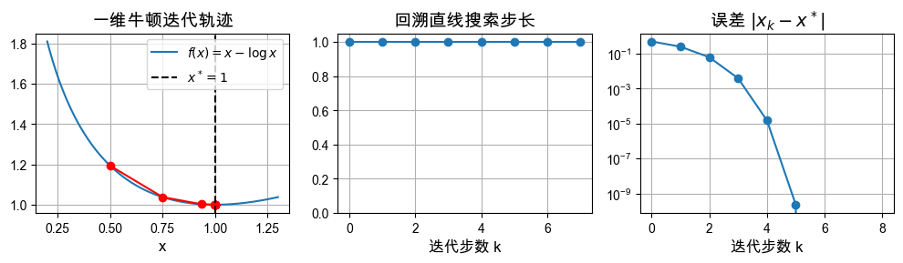
观察结果：

从 $x^{(0)}=0.5$ 出发时，回溯直线搜索会持续接受 $t=1$ ，因此算法一直处于纯牛顿阶段。
误差满足 $e_{k+1}\approx e_k^2$ ，这正是课件里强调的二次收敛现象。
这个例子说明：当局部二次模型很准确时，牛顿法会非常快。

例子2：二维二次函数¶

现在回到二维问题，比较梯度法和牛顿法在一个标准凸二次函数上的表现。

对于二次函数，Hessian 是常数矩阵，因此牛顿法应该非常有优势。

gamma = 10.0
f = lambda x: (x[0]**2 + gamma * x[1]**2) / 2
df = lambda x: np.array([x[0], gamma * x[1]])
hessian = lambda x: np.array([[1.0, 0.0], [0.0, gamma]])

prob = Problem(f=f, df=df, hessian=hessian)
prob.alpha = 0.05
prob.beta = 0.7
prob.tol = 1.0e-8

x0 = np.array([9.0, 2.0])
xmin, xmax, ymin, ymax = -5, gamma, -5, 5

prob.method = 'gradient'
trajectory_gd, runtime_gd, t_list_gd, _ = prob.solve(x0)

prob.method = 'newton'
trajectory_newton, runtime_newton, t_list_newton, decrement_list = prob.solve(x0)

print_large(f'梯度法运行时间：{runtime_gd * 1e3:.2f} ms')
print_large(f'牛顿法运行时间：{runtime_newton * 1e3:.2f} ms')
print_large(f'梯度法迭代步数：{len(trajectory_gd) - 1}')
print_large(f'牛顿法迭代步数：{len(trajectory_newton) - 1}')
print_large(f'牛顿减量初值：{decrement_list[0]:.3e}')

plt.figure(figsize=(11, 3.8))

plt.subplot(1, 3, 1)
plt.plot(trajectory_gd[:, 0], trajectory_gd[:, 1], 'rx-', label='梯度法')
plt.plot(trajectory_newton[:, 0], trajectory_newton[:, 1], 'bo-', label='牛顿法')
prob.plot_contour(xmin, xmax, ymin, ymax)
plt.title('二维二次函数上的迭代轨迹', fontsize=14)
plt.legend(fontsize=10)

plt.subplot(1, 3, 2)
plt.plot(np.linalg.norm(trajectory_gd, ord=2, axis=1), 'rx-', label='梯度法')
plt.plot(np.linalg.norm(trajectory_newton, ord=2, axis=1), 'bo-', label='牛顿法')
plt.yscale('log')
plt.title('误差 $|x_k-x^*|_2$', fontsize=14)
plt.xlabel('迭代步数 k', fontsize=12)
plt.grid()
plt.legend(fontsize=10)

plt.subplot(1, 3, 3)
plt.plot(range(len(t_list_gd)), t_list_gd, 'rx-', label='梯度法')
plt.plot(range(len(t_list_newton)), t_list_newton, 'bo-', label='牛顿法')
plt.title('回溯直线搜索步长', fontsize=14)
plt.xlabel('迭代步数 k', fontsize=12)
plt.ylim(0, 1.05)
plt.grid()
plt.legend(fontsize=10)

plt.tight_layout()
plt.show()

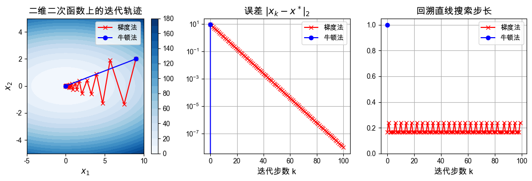
观察结果：

在二次函数上，牛顿法几乎立即到达极小值点。
这是因为这个问题的二阶模型就是原函数本身，牛顿步直接抓住了正确曲率。
梯度法虽然也收敛，但会经历明显更多的迭代。

例子3：二维非二次函数¶

下面的函数不是二次函数，因此牛顿法不可能一步到达最优解。

但如果理论成立，那么当迭代进入真解附近后，仍然应该看到明显快于梯度法的局部收敛。

f(x,y)=e^{x+3y-0.1}+e^{x-3y-0.1}+e^{-x-0.1}.

(2)

f = lambda x: np.exp(x[0] + 3 * x[1] - 0.1) + np.exp(x[0] - 3 * x[1] - 0.1) + np.exp(-x[0] - 0.1)
df = lambda x: np.array([
    np.exp(x[0] + 3 * x[1] - 0.1) + np.exp(x[0] - 3 * x[1] - 0.1) - np.exp(-x[0] - 0.1),
    3 * np.exp(x[0] + 3 * x[1] - 0.1) - 3 * np.exp(x[0] - 3 * x[1] - 0.1)
])
hessian = lambda x: np.array([
    [
        np.exp(x[0] + 3 * x[1] - 0.1) + np.exp(x[0] - 3 * x[1] - 0.1) + np.exp(-x[0] - 0.1),
        3 * np.exp(x[0] + 3 * x[1] - 0.1) - 3 * np.exp(x[0] - 3 * x[1] - 0.1)
    ],
    [
        3 * np.exp(x[0] + 3 * x[1] - 0.1) - 3 * np.exp(x[0] - 3 * x[1] - 0.1),
        9 * np.exp(x[0] + 3 * x[1] - 0.1) + 9 * np.exp(x[0] - 3 * x[1] - 0.1)
    ]
])

prob = Problem(f=f, df=df, hessian=hessian)
prob.alpha = 0.1
prob.beta = 0.1

x0 = np.array([1.0, 1.0])
xmin, xmax, ymin, ymax = -1, 2, -1, 1.5

# 先用高精度牛顿法求一个近似最优解，用于后续误差作图。
prob.tol = 1.0e-20
prob.method = 'newton'
trajectory_ref, runtime_ref, _, _ = prob.solve(x0, max_iter=50)
x_star = trajectory_ref[-1]
p_star = prob.f(x_star)

# 再按常规容差比较梯度法和牛顿法。
prob.tol = 1.0e-10

prob.method = 'gradient'
trajectory_gd, runtime_gd, t_list_gd, _ = prob.solve(x0, max_iter=100)

prob.method = 'newton'
trajectory_newton, runtime_newton, t_list_newton, decrement_list = prob.solve(x0, max_iter=100)

gd_error = np.array([max(prob.f(item) - p_star, 1.0e-16) for item in trajectory_gd])
newton_error = np.array([max(prob.f(item) - p_star, 1.0e-16) for item in trajectory_newton])
safe_mask = newton_error[:-1] < 0.5
loglog_indices = np.where(safe_mask)[0]
loglog_error = np.log2(np.log2(1.0 / newton_error[:-1][safe_mask]))

print_large(f'近似最优解计算时间：{runtime_ref * 1e3:.2f} ms')
print_large(f'梯度法运行时间：{runtime_gd * 1e3:.2f} ms')
print_large(f'牛顿法运行时间：{runtime_newton * 1e3:.2f} ms')
print_large(f'梯度法迭代步数：{len(trajectory_gd) - 1}')
print_large(f'牛顿法迭代步数：{len(trajectory_newton) - 1}')
print_large(f'参考近似解 x^* = [{x_star[0]:.2f}, {x_star[1]:.2f}]')

plt.figure(figsize=(12, 6))

plt.subplot(2, 2, 1)
plt.plot(trajectory_gd[:, 0], trajectory_gd[:, 1], 'rx-', label='梯度法')
plt.plot(trajectory_newton[:, 0], trajectory_newton[:, 1], 'bo-', label='牛顿法')
prob.plot_contour(xmin, xmax, ymin, ymax)
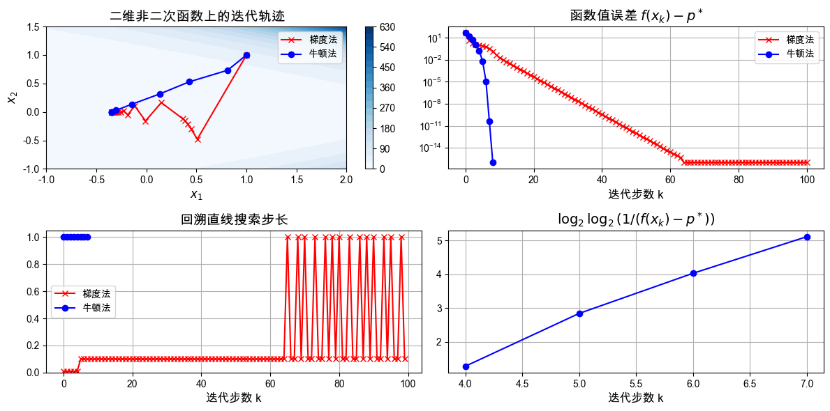
plt.title('二维非二次函数上的迭代轨迹', fontsize=14)
plt.legend(fontsize=10)

plt.subplot(2, 2, 2)
plt.plot(gd_error, 'rx-', label='梯度法')
plt.plot(newton_error, 'bo-', label='牛顿法')
plt.yscale('log')
plt.title(r'函数值误差 $f(x_k)-p^*$', fontsize=14)
plt.xlabel('迭代步数 k', fontsize=12)
plt.grid()
plt.legend(fontsize=10)

plt.subplot(2, 2, 3)
plt.plot(range(len(t_list_gd)), t_list_gd, 'rx-', label='梯度法')
plt.plot(range(len(t_list_newton)), t_list_newton, 'bo-', label='牛顿法')
plt.title('回溯直线搜索步长', fontsize=14)
plt.xlabel('迭代步数 k', fontsize=12)
plt.ylim(0, 1.05)
plt.grid()
plt.legend(fontsize=10)

plt.subplot(2, 2, 4)
plt.plot(loglog_indices, loglog_error, 'bo-')
plt.title(r'$\log_2\log_2(1/(f(x_k)-p^*))$', fontsize=14)
plt.xlabel('迭代步数 k', fontsize=12)
plt.grid()

plt.tight_layout()
plt.show()

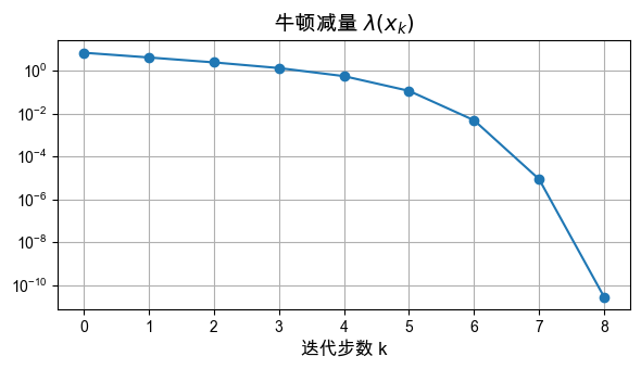
print_large("\n\n牛顿减量变化情况：\n\n")

plt.figure(figsize=(6, 3.5))
plt.plot(decrement_list, 'o-')
plt.yscale('log')
plt.title(r'牛顿减量 $\lambda(x_k)$', fontsize=14)
plt.xlabel('迭代步数 k', fontsize=12)
plt.grid()
plt.tight_layout()
plt.show()

观察结果：

在非二次函数上，牛顿法不再一步到达最优点，但迭代次数仍明显少于梯度法。
当迭代进入真解附近后，函数值误差下降得非常快，这和局部二次收敛的理论一致。
$\log \log(1/e_k)$ 图像近似线性，是课件中理论结论的一个数值迹象。
牛顿减量逐步变小，也说明算法正在逼近局部最优点。

总结¶

这个 notebook 验证或强调了三件事：

牛顿法本质上是在利用当前点附近的二阶信息修正梯度方向。
实际实现中通常采用阻尼牛顿法，即“牛顿方向 + 回溯直线搜索”。
一旦进入纯牛顿阶段，误差往往会呈现 $e_{k+1}\approx C e_k^2$ 的局部二次收敛。

学习目标¶

例子1：一维函数 f(x)=x−ln⁡xf(x)=x-\ln xf(x)=x−lnx¶

例子2：二维二次函数¶

例子3：二维非二次函数¶

总结¶

例子1：一维函数 $f(x)=x-\ln x$ ¶