第5章 Newton-Cotes

import numpy as np
import matplotlib.pyplot as plt
import pandas as pd

def trapezoidal(a, b, n, f):
    h = (b-a)/n
    x = np.linspace(a, b, num=n+1, endpoint=True)
    s = 0.0
    for i in range(n):
        s = s + 0.5 * h *(f(x[i])+f(x[i+1]))
    return s

def simpson(a, b, n, f):
    h = (b-a)/n
    x = np.linspace(a, b, num=n+1, endpoint=True)
    s = 0.0
    for i in range(n):
        s = s + h / 6 *(f(x[i]) + 4*f(x[i]/2+x[i+1]/2) + f(x[i+1]))
    return s

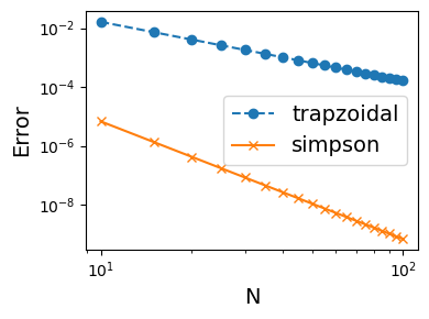
测试对\(\sin\)函数的积分

f = lambda x : np.sin(x)
a = 0
b = np.pi
exact_value = 2

n_list = np.array(range(10, 105, 5))
err_list_trap = np.zeros(len(n_list))
err_list_simpson = np.zeros(len(n_list))
for n_idx in range(len(n_list)):
    n = n_list[n_idx]
    err_list_trap[n_idx] = np.abs(trapezoidal(a, b, n, f) - exact_value)
    err_list_simpson[n_idx] = np.abs(simpson(a, b, n, f) - exact_value)

plt.figure(figsize=(4,3))
plt.plot(n_list, err_list_trap, 'o--', label="trapzoidal")
plt.plot(n_list, err_list_simpson, 'x-', label="simpson")
plt.legend(fontsize=14)
plt.yscale('log')
plt.xscale('log')
plt.xlabel('N',fontsize=14)
plt.ylabel('Error',fontsize=14)
plt.tight_layout()

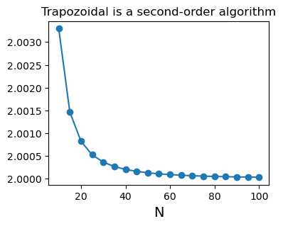
验证课本的对于复化梯形法的误差公式(4.2.15)

plt.figure(figsize=(4,3))
plt.plot(n_list, err_list_trap / (((b-a)/n_list)**2/12), 'o-')
plt.title('Trapozoidal is a second-order algorithm')
plt.xlabel('N',fontsize=14)
plt.show()

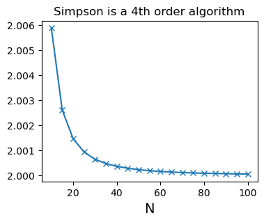
验证课本的对于复化Simpson的误差公式(4.2.16)

plt.figure(figsize=(4,3))
plt.plot(n_list, err_list_simpson / ((((b-a)/n_list)**4) / 180 / 2**4), 'x-')
plt.title('Simpson is a 4th order algorithm')
plt.xlabel('N',fontsize=14)
plt.show()

Roomberg算法

def Roomberg(a, b, n, f):
    Ttable = np.zeros((n+1, n+1)) * np.nan
    for k in range(n+1):
        for m in range(k+1):
            if m == 0:
                Ttable[k,m] = trapezoidal(a, b, 2**k, f)
            else:
                alpha = 4**m
                Ttable[k,m] = alpha/(alpha-1)*Ttable[k,m-1] - 1/(alpha-1)*Ttable[k-1,m-1]
    return Ttable

f = lambda x : np.sin(x)
a = 0
b = np.pi
n = 6
Ttable = Roomberg(a, b, n, f)
pd.DataFrame(Ttable)

	0	1	2	3	4	5	6
0	1.923671e-16	NaN	NaN	NaN	NaN	NaN	NaN
1	1.570796e+00	2.094395	NaN	NaN	NaN	NaN	NaN
2	1.896119e+00	2.004560	1.998571	NaN	NaN	NaN	NaN
3	1.974232e+00	2.000269	1.999983	2.000006	NaN	NaN	NaN
4	1.993570e+00	2.000017	2.000000	2.000000	2.0	NaN	NaN
5	1.998393e+00	2.000001	2.000000	2.000000	2.0	2.0	NaN
6	1.999598e+00	2.000000	2.000000	2.000000	2.0	2.0	2.0

pd.DataFrame(np.abs(Ttable-2.0)).map(lambda x: f"{x:.2e}")

	0	1	2	3	4	5	6
0	2.00e+00	nan	nan	nan	nan	nan	nan
1	4.29e-01	9.44e-02	nan	nan	nan	nan	nan
2	1.04e-01	4.56e-03	1.43e-03	nan	nan	nan	nan
3	2.58e-02	2.69e-04	1.69e-05	5.55e-06	nan	nan	nan
4	6.43e-03	1.66e-05	2.48e-07	1.63e-08	5.41e-09	nan	nan
5	1.61e-03	1.03e-06	3.81e-09	5.97e-11	3.97e-12	1.32e-12	nan
6	4.02e-04	6.45e-08	5.93e-11	2.29e-13	4.00e-15	2.22e-16	6.66e-16

# 例子4.3的表格

def sinx_divide_x(x):
    if x < 1.0e-5:
        return 1
    else:
        return np.sin(x)/x
    
f = lambda x : sinx_divide_x(x)

a = 0
b = 1
n = 4

pd.DataFrame(Roomberg(a, b, n, f))

	0	1	2	3	4
0	0.920735	NaN	NaN	NaN	NaN
1	0.939793	0.946146	NaN	NaN	NaN
2	0.944514	0.946087	0.946083	NaN	NaN
3	0.945691	0.946083	0.946083	0.946083	NaN
4	0.945985	0.946083	0.946083	0.946083	0.946083