第3.4章 解线性方程迭代法#
from scipy.sparse import random
import matplotlib.pyplot as plt
import scipy
import numpy as np
(1) 对于稀疏矩阵,直接的LU分解无法合理利用稀疏性质#
np.random.seed(1)
n = 1000
A = random(n,n,0.02).toarray()
A += np.diag(2*np.sum(A, axis=1))
b = np.random.randn(n)
P, L, U = scipy.linalg.lu(A)
print("A矩阵的非零项比例为:{:.3f}\n".format(sum(sum(1.0*(A != 0)))/n**2))
print("L矩阵的非零项比例为:{:.3f}".format(sum(sum(1.0*(L != 0)))/n**2))
print("U矩阵的非零项比例为:{:.3f}".format(sum(sum(1.0*(U != 0)))/n**2))
A矩阵的非零项比例为:0.021

L矩阵的非零项比例为:0.410
U矩阵的非零项比例为:0.406
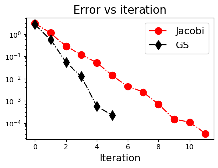
(2) 课本内的三维的例子#
def jacobi(A, b, max_iterations=100, tolerance=1e-6):
    """
        Jacobi 迭代法
    """
    n = len(b)
    x = np.random.randn(n)  # Initial guess
    err = np.zeros(max_iterations)

    for k in range(max_iterations):
        x_old = x.copy()
        for i in range(n):
            sigma = sum(A[i, j] * x_old[j] for j in range(n) if j != i)
            x[i] = (b[i] - sigma) / A[i, i]

        # Check convergence
        err[k] = np.linalg.norm(x - x_old, ord=np.inf)
        if  err[k] < tolerance:
            print(f'Converged in {k + 1} iterations.')
            return x, err[0:k], k

    print(f'Warning: Did not converge after {max_iterations} iterations.')
    return x, err[0:k], k

def gauss_seidel(A, b, initial_guess=None, max_iterations=100, tolerance=1e-6):
    """
       Gauss-Seidel 迭代法
    """
    n = len(b)
    x = initial_guess if initial_guess is not None else np.random.randn(n)
    err = np.zeros(max_iterations)

    for k in range(max_iterations):
        for i in range(n):
            x_old_item = x[i]
            sigma_forward = np.dot(A[i, :i], x[:i])  # Forward substitution
            sigma_backward = np.dot(A[i, (i+1):], x[(i+1):])  # Backward substitution
            x[i] = (b[i] - sigma_forward - sigma_backward) / A[i,i]

            # use inf-norm
            err[k] = np.maximum(err[k], np.abs(x[i] - x_old_item))

        # Check convergence
        if err[k] < tolerance:
            print(f'Converged in {k + 1} iterations.')
            return x, err[0:k], k

    print(f'Warning: Did not converge after {max_iterations} iterations.')
    return x, err[0:k], k

def SOR(A, b, ω, initial_guess=None, max_iterations=100, tolerance=1e-6):
    """
        逐次超松弛迭代法
    """
    n = len(b)
    x = initial_guess if initial_guess is not None else np.random.randn(n)
    err = np.zeros(max_iterations)

    for k in range(max_iterations):
        for i in range(n):
            x_old_item = x[i]
            sigma_forward = np.dot(A[i, :i], x[:i])  # Forward substitution
            sigma_backward = np.dot(A[i, (i+1):], x[(i+1):])  # Backward substitution
            x[i] = (b[i] - sigma_forward - sigma_backward) / A[i,i]
            x[i] = ω * x[i] + (1-ω)*x_old_item

            # use inf-norm
            err[k] = np.maximum(err[k], np.abs(x[i] - x_old_item))

        # Check convergence
        if err[k] < tolerance:
            print(f'Converged in {k + 1} iterations.')
            return x, err[0:k], k

    print(f'Warning: Did not converge after {max_iterations} iterations.')
    return x, err[0:k], k
# 课本例题8.1

A = np.array([[8.0, -3, 2], [4, 11, -1], [6, 3, 12]])
b = np.array([20,33,36])

np.random.seed(1)
x_jac, err_jac, k_jac = jacobi(A.copy(), b.copy(), tolerance=1.0e-5)
print(x_jac)

np.random.seed(1)
x_gs, err_gs, k_gs = gauss_seidel(A.copy(), b.copy(), tolerance=1.0e-5)
print(x_gs)

plt.figure(figsize=(4.5,3.5))
plt.plot(range(k_jac), err_jac, 'ro-.', markersize=10.0, label="Jacobi")
plt.plot(range(k_gs),  err_gs,  'kd-.', markersize=10.0, label="GS")
plt.yscale("log")
plt.xlabel("Iteration", fontsize=14)
plt.title("Error vs iteration", fontsize=16)
plt.legend(fontsize=14)
plt.tight_layout()
plt.show()
Converged in 13 iterations.
[2.99999782 2.00000464 1.00000492]
Converged in 7 iterations.
[3.0000029  1.99999831 0.99999897]
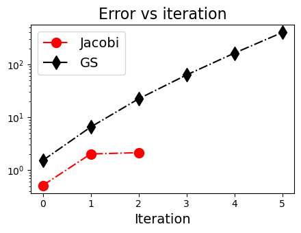
(3) GS迭代法不一定比Jacobi迭代法好#
# 课本例题 8.3

A = np.array([[1.0, 2, -2], [1, 1, 1], [2, 2, 1]])
b = np.array([1, 1, 1])
x_true = np.linalg.solve(A, b)

np.random.seed(1)
x_jac, err_jac, k_jac = jacobi(A.copy(), b.copy(), tolerance=1.0e-5, max_iterations=7)
print(x_jac)

np.random.seed(1)
x_gs, err_gs, k_gs = gauss_seidel(A.copy(), b.copy(), tolerance=1.0e-5, max_iterations=7)
print(x_gs)

plt.figure(figsize=(4.5,3.5))
plt.plot(range(k_jac), err_jac, 'ro-.', markersize=10.0, label="Jacobi")
plt.plot(range(k_gs),  err_gs,  'kd-.', markersize=10.0, label="GS")
plt.yscale("log")
plt.xlabel("Iteration", fontsize=14)
plt.title("Error vs iteration", fontsize=16)
plt.legend(fontsize=14)
plt.tight_layout()
plt.show()
Converged in 4 iterations.
[-3.  3.  1.]
Warning: Did not converge after 7 iterations.
[-1496.75502195  1594.55801409  -194.60598429]
print("Error of Jacobi = {:.3f}".format(np.linalg.norm(x_jac - x_true)))
print(x_jac)
print(x_true)
Error of Jacobi = 0.000
[-3.  3.  1.]
[-3.  3.  1.]
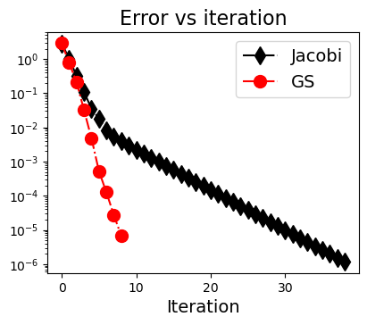
(4) 高维问题#
np.random.seed(4)
n = 100
A = random(n,n,0.1).toarray()
A += np.diag(1.3 * np.sum(A, axis=1))
b = np.random.randn(n)
seed = 4

np.random.seed(seed)
x_jac, err_jac, k_jac = jacobi(A, b, tolerance=1.0e-6)
np.random.seed(seed)
x_gs,  err_gs,  k_gs  = gauss_seidel(A, b, tolerance=1.0e-6)

plt.figure(figsize=(4.5,3.5))
plt.plot(range(k_jac), err_jac, 'kd-.', markersize=10.0, label="Jacobi")
plt.plot(range(k_gs),  err_gs,  'ro-.', markersize=10.0, label="GS")
plt.yscale("log")
plt.xlabel("Iteration", fontsize=14)
plt.title("Error vs iteration", fontsize=16)
plt.legend(fontsize=14)
plt.show()
Converged in 40 iterations.
Converged in 10 iterations.
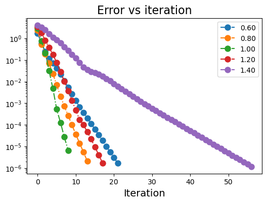
plt.figure(figsize=(6,4))
ω_list = [0.6, 0.8, 1.0, 1.2, 1.4]
for j in range(len(ω_list)):
    ω = ω_list[j]
    np.random.seed(seed)
    x_sor, err_sor, k_sor = SOR(A.copy(), b.copy(), ω)
    plt.plot(range(k_sor), err_sor, 'o-.', markersize=8.0, label="{:.2f}".format(ω))

plt.yscale("log")
plt.legend()
plt.xlabel("Iteration", fontsize=14)
plt.title("Error vs iteration", fontsize=16)
plt.show()
Converged in 23 iterations.
Converged in 15 iterations.
Converged in 10 iterations.
Converged in 19 iterations.
Converged in 58 iterations.
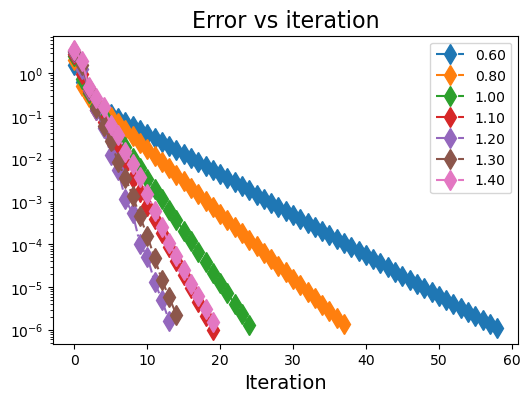
(5) 对于\(\omega\)的优化#
# 课本例子 8.11

seed = 5
n = 4
A = np.array([[-4,1,1,1],[1,-4,1,1],[1,1,-4,1],[1,1,1,-4]])
b = np.array([1,1,1,1])

plt.figure(figsize=(6,4))
ω_list = [0.6, 0.8, 1.0, 1.1, 1.2, 1.3, 1.4]
for j in range(len(ω_list)):
    ω = ω_list[j]
    np.random.seed(seed)
    x_sor, err_sor, k_sor = SOR(A.copy(), b.copy(), ω, tolerance=1e-6)
    plt.plot(range(k_sor), err_sor, 'd-.', markersize=10.0, label="{:.2f}".format(ω))

plt.yscale("log")
plt.legend()
plt.xlabel("Iteration", fontsize=14)
plt.title("Error vs iteration", fontsize=16)
plt.show()
Converged in 60 iterations.
Converged in 39 iterations.
Converged in 26 iterations.
Converged in 21 iterations.
Converged in 15 iterations.
Converged in 16 iterations.
Converged in 21 iterations.
from numpy import linalg as LA

B0 = np.identity(n)- np.matmul(np.linalg.inv(np.diag(np.diag(A))), A)
value = LA.eigvals(B0)
rho = np.max(np.abs(value))
ω_best = 2/(1+np.sqrt(1-rho**2))
print("spectral radius = {:.2f}".format(rho))
print("best omega      = {:.2f}".format(ω_best))
spectral radius = 0.75
best omega      = 1.20
A = np.array([[-4,1,1,1],[1,-4,1,1],[1,1,-4,1],[1,1,1,-4]])
U = -np.array([[0,1,1,1],[0,0,1,1],[0,0,0,1],[0,0,0,0]])
L = -np.array([[0,0,0,0],[1,0,0,0],[1,1,0,0],[1,1,1,0]])
D = np.diag(np.diag(A))

ω = 1.1
Lomega = np.matmul(np.linalg.inv(D - ω * L), (1-ω) * D + ω * U)
spec_radius = np.max(np.abs(LA.eigvals(Lomega)))
print("omega = {:.2f} spec_radius = {:.2f}".format(ω, spec_radius))

ω = 1.2
Lomega = np.matmul(np.linalg.inv(D - ω * L), (1-ω) * D + ω * U)
spec_radius = np.max(np.abs(LA.eigvals(Lomega)))
print("omega = {:.2f} spec_radius = {:.2f}".format(ω, spec_radius))

ω = 1.3
Lomega = np.matmul(np.linalg.inv(D - ω * L), (1-ω) * D + ω * U)
spec_radius = np.max(np.abs(LA.eigvals(Lomega)))
print("omega = {:.2f} spec_radius = {:.2f}".format(ω, spec_radius))
omega = 1.10 spec_radius = 0.48
omega = 1.20 spec_radius = 0.33
omega = 1.30 spec_radius = 0.37